Machine learning classification based on \(k\)-Nearest Neighbors for PolSAR data
Programa de Pós-Graduação em Estatística
Prof. Dr. Jodavid Ferreira
UFPE
![]()
Who is Dr. Jodavid Ferreira?
- Bachelor’s degree in Statistics from UFPB;
- Master’s degree in Statistics from UFPE;
- PhD in Statistics from UFPE;
Research Experiences
- Statistical Machine Learning;
- Image Processing;
- Fuzzy Probability
Professional Experience
- HartB Group and ThinkAI Group (Startups focused on Artificial Intelligence);
- Certified in AI by Huawei and in Data Engineering by Google;
Structure of the presentation
- Different versions of \(k\)-NN;
About paper
Publication on Annals of the Brazilian Academy of Sciences:
Machine learning classification based on \(k\)-Nearest Neighbors for PolSAR data
Authors: Ferreira, J.A. & Rodrigues, A.K.G. & Ospina, R. & Gomez, L.
Year: 2024 - DOI:10.1590/0001-3765202420230064
![]()
Notation
- \(X\) or \(Y\)
- \(x\) or \(y\)
- \(\mathbf{x}\) or \(\mathbf{y}\)
- \(\dot{\mathbf{x}}\) or \(\dot{\mathbf{y}}\)
- \(\mathbf{X}\) or \(\mathbf{Y}\)
- \(\dot{\mathbf{X}}\) or \(\dot{\mathbf{Y}}\)
represent random variables (r.v.);
represent realizations of random variables;
represent random vectors;
represent realizations of random vectors;
represent random matrices;
represent realizations of random matrices;
dimension of features, variables, parameters
sample size
\(i\)-th observation, instance (e.g., \(i=1, ..., n\))
\(j\)-th feature, variable, parameter (e.g., \(j=1, ..., p\))
Introduction
- RADAR is an acronym of Radio Detection and Ranging
- It is based on the principles of electromagnetic propagation, in which an electromagnetic wave is emitted by a source and is backscattered to radar
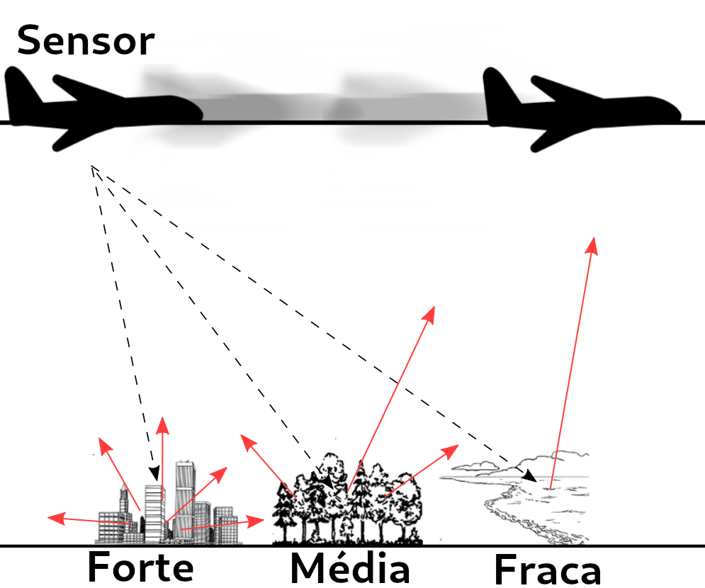
- According to Zyl (2011), a radar image is the result of an interaction between the energy launched by the radar and the object under study and the appearance of the image is influenced by the shape and texture of the target
Introduction
- Synthetic Aperture Radar (SAR) is coupled to a platform that transmits microwaves along its intended route towards a geographic scene;
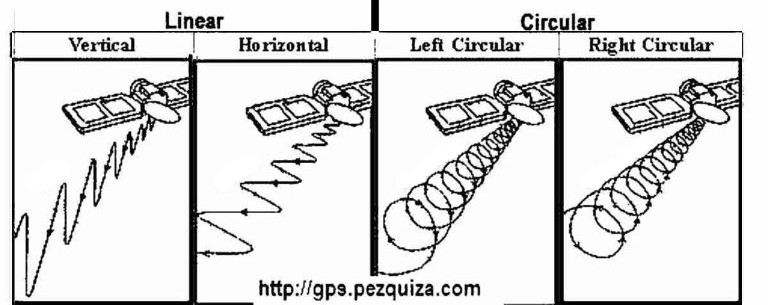
- Pulses emitted towards a real scenario may have circular and/or linear polarizations;
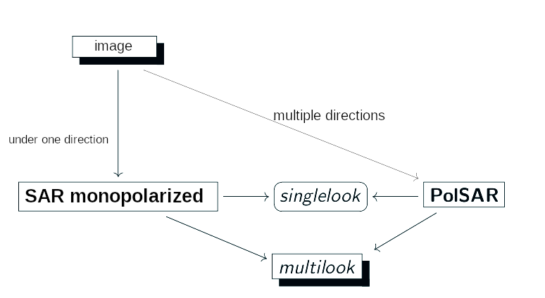
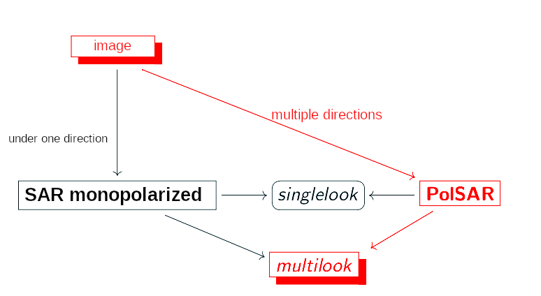
- When only one pair of directions is used, the images generated are called monopolarized SAR and, when multiple directions are used, the process is called PolSAR (Polarimetric SAR);
Introduction
![]()
Introduction
![]()
Introduction
Advantages
- SAR images can be obtained in from anywhere (land, sea, air);
- at any time (day or night);
- in almost all weather conditions (clouds, rain);
- produce high-resolution (high-bandwidth) images of the surfaces studied;
Disadvantages
- high cost;
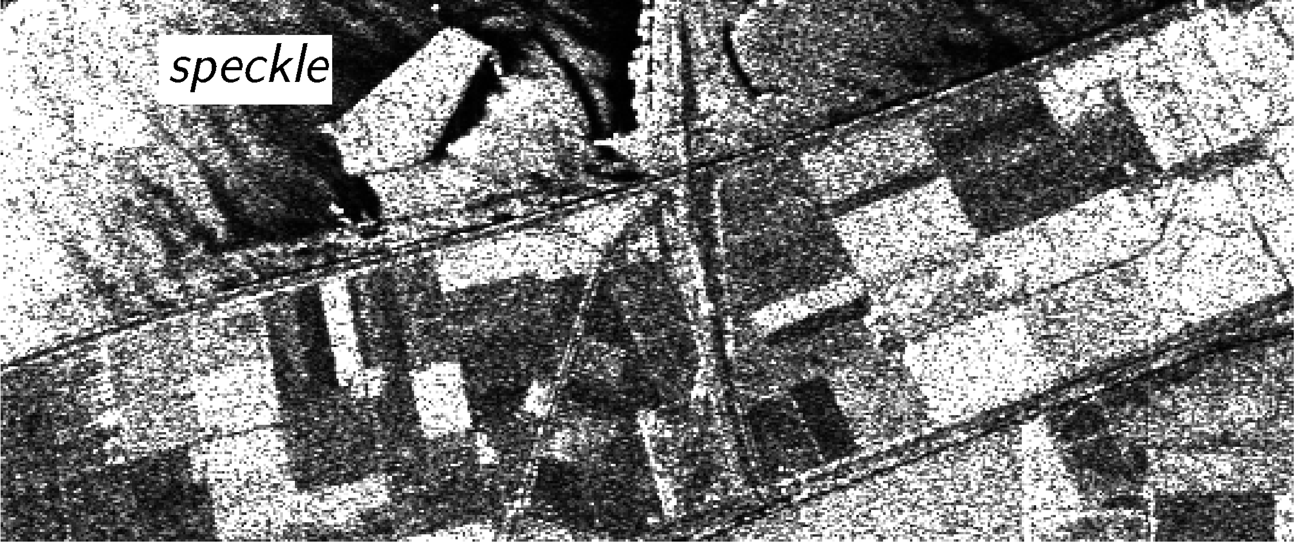
- the images obtained are affected by a noise called speckle, which creates a granular appearance in the images, making interpretation and analysis difficult;
Introduction
Advantages
- SAR images can be obtained in from anywhere (land, sea, air);
- at any time (day or night);
- in almost all weather conditions (clouds, rain);
- produce high-resolution (high-bandwidth) images of the surfaces studied;
Disadvantages
- high cost;
- the images obtained are affected by a noise called speckle, which creates a granular appearance in the images, making interpretation and analysis difficult;
Introduction
![]()
Speckle in SAR image. Source: (NASCIMENTO, 2012).
Introduction
Speckle imposes on SAR/PolSAR data a multiplicative nature such that SAR intensities or multidimensional intensities of a given PolSAR do not behave like the normal or Gaussian law.
Methods considering speckle action have been proposed in several areas:
- Classification;
- Segmentation;
- Edge detection;
- Change detection;
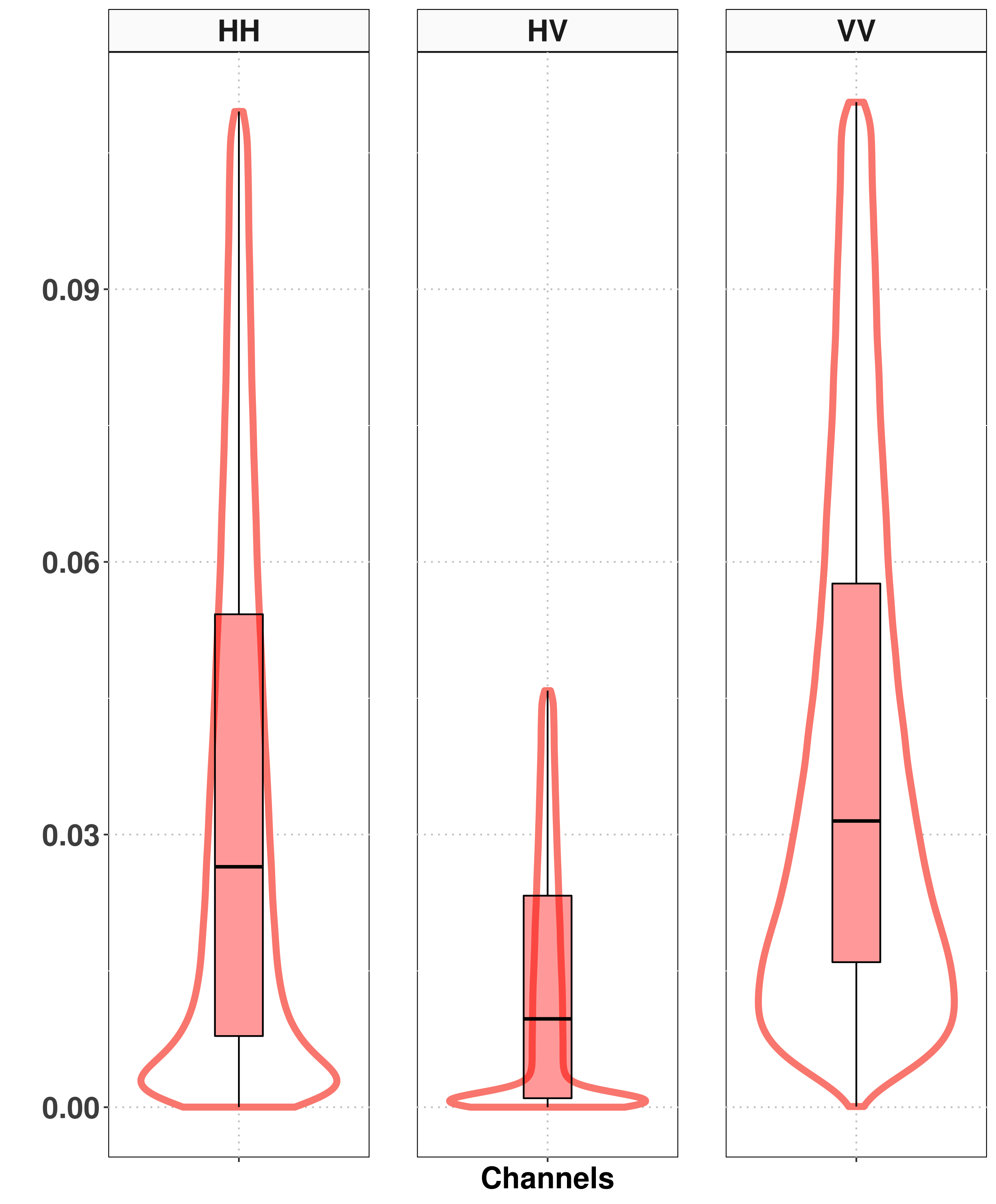
Polarimetric Data multi-look
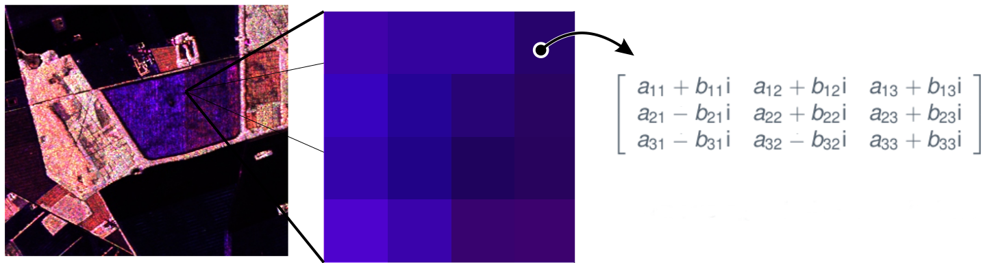
- PolSAR image is such that each entry is associated with the elements of the following matrix:
\[
\mathbf{S}=\left( \begin{array}{cc}
S_{hh} & S_{hv} \\
S_{vh} & S_{vv} \end{array} \right)
\label{matrizpolar}
\]
- In practice, the cross-polarizations are very similar; that is, \(S_{hv} \approx S_{vh}\). Thus, the above matrix can be represented as
\[
\mathbf{z}=\left( \begin{array}{c}
S_{hh}\\
S_{hv}\\
S_{vv} \end{array} \right)
\label{matrizpolarreduzida}
\]
Polarimetric Data multi-look
- PolSAR data single-look don’t take into account the control of the speckle effect on images
- A process to circumvent this is called multi-look processing
Polarimetric Data multi-look
\(\mathbf{z}_i = (S_1^{(i)}\,S_2^{(i)}\,\cdots\,S_p^{(i)})^{\top} \, \in \mathbb{C}^{p}\) is the \(i\)-th vector associated with \(p\) polarization channels in a sample of \(L\) extracted information from the same scene, for \(i=1,\ldots,L\).
![]()
Polarimetric Data multi-look
- A PolSAR image can be understood as a scene, in which each entry is associated with a positive definite Hermitian matrix, which requires the use of multivariate processing methods.
![]()
Machine Learning Classifiers
- Machine learning (ML) is a huge interdisciplinary area of research focusing on solving problems from knowledge from data.
- Classifiers based on Nearest Neighbors:
- k-NN classifier;
- Kernel k-NN classifier;
- Fuzzy k-NN classifier;
- Fuzzy Kernel k-NN classifier;
- Support Vector Machine (SVM);
- Extreme Gradient Boosting (XGBoost);
- Naive Bayes;
- The Kullback-Leibler classifier;
k-NN classifier
- The \(k\)-Nearest Neighbors algorithm is an extension of the NN algorithm and was proposed by Cover e Hart (1967) and is considered as a non-parametric classifier.
- Given a test sample where the class is unknown, the method finds the nearest \(k\) in the training set for each observation of the test sample over a distance and assigns a class to the observation according to the majority vote of the classes of these neighbors.
- Let \(\mathbf{x}_1 = [x_{11},x_{12},\ldots,x_{1p} ]^{\top}\) and \(\mathbf{x}_2 = [x_{21},x_{22},\ldots,x_{2p} ]^{\top}\) two vectors \(p\)-dimensional, in which, \(^{\top}\) represents the transposed operator, the similarity between \(\mathbf{x}_1\) and \(\mathbf{x}_2\) is measured by the Euclidean distance is obtained as:
\[
d(\mathbf{x}_1,\mathbf{x}_2) = \parallel \mathbf{x}_1 - \mathbf{x}_2 \parallel
= \sqrt{\sum\limits_{j=1}^{p}(x_{1j} - x_{2j})^2}.
\]
k-NN classifier
- The algorithm \(k\)-NN estimates the probability of an observation belonging to each group based on the nearest neighbor \(k\) information defined as follows.
Consider \(G\) non-empty partitions, which are \(C_1,C_2, \ldots,C_c\), such that, \(C_t \subset \mathbb{R}^p\) is a subset of size \(n_t\), for \(t = 1, \ldots,c\), \(n = \sum_{t=1}^{c} n_t\), \(C_u\cap C_v = \emptyset\) for all \(u \neq v.\)
Let \(\mathbf{x}_r \in \mathbb{R}^p\) an observation to be classified, where \(r \notin 1, \ldots, n\) and \(\{\mathbf{x}_{i_1},\mathbf{x}_{i_2},\ldots,\mathbf{x}_{i_k} \}\) the set of \(k\) neighbors, such that, \(k\leq n\) and \(\{{i_1},{i_2},\ldots,{i_k} \} \subset \{1,2,\ldots,n\}\). So for \(t = 1, \ldots,c\), the classification rule of the \(k\)-NN is defined as:
\[\begin{equation}
\widehat{c}_{_{kNN}} = \underset{c}{\mathrm{arg max}} \ \widehat{P}_k(c | \mathbf{x}_r),
\end{equation}\]
where \(\widehat{P}_k(c | \mathbf{x}_r) = k^{-1}\sum_{\nu=1}^{k}\mathbb{I}_c(\mathbf{x}_{i_\nu})\) and
\[\begin{eqnarray}
\mathbb{I}_c(\mathbf{x}_{i_\nu}) = \left\{
\begin{array}{rl}
1,&\text{if } \mathbf{x}_{i_\nu} \in C_j,\\
0,& \text{if } \mathbf{x}_{i_\nu} \notin C_j.
\end{array}
\right. \nonumber
\end{eqnarray}\]
Kernel k-NN classifier
The kernel k-NN classifier is a natural extension of the \(k\)-NN algorithm in which the training samples are transformed into a feature space through a nonlinear transformation.
Thus, consider a transformation in the \(p\)-dimensional feature space for a \(s\)-dimensional feature space (usually with \(p \leq s\)), in which, given an arbitrary vector \(\mathbf{x} \in E_1\) (original \(p\)-dimensional feature space), with \(\psi(\mathbf{x})\) being the respective vector in \(E_2\) (new \(s\)-dimensional feature space), the transformation is obtained as follows:
\[\begin{eqnarray}
\begin{array}{c}
\mathbf{x} = (x_1,x_2,\ldots, x_p), \quad\quad \mathbf{x} \in E_1\\
\quad\quad\quad\quad
\quad\quad\quad\quad
\Bigg\downarrow ( \text{transformation of characteristics})\\
\psi(\mathbf{x}) = \left(\phi_1(\mathbf{x}),\phi_2(\mathbf{x}), \ldots, \phi_s(\mathbf{x})\right), \quad\quad \psi(\mathbf{x}) \in E_2 \\
\end{array}
\label{transformation_of_char}
\end{eqnarray}\]
Kernel k-NN classifier
- Given \(\mathbf{x} \in E_1 \subseteq \mathbb{R}^p\) the vector of characteristics of the original data and \(\psi\) a non-linear continuous, symmetric and positive semi-definite transformation of \(E_1\) for a possible space of high dimension \(E_2\) (Hilbert space). The transformation of \(\mathbf{x}\) for \(\psi\) represents the space of characteristics.
- To use \(k\)-NN in a space of high-dimensional characteristics, it is necessary that the classification process is executed in such space.
- A kernel can be defined as a \(K\) function, such that,
\[\begin{equation}
K(\mathbf{x}_1,\mathbf{x}_2) = \langle \psi(\mathbf{x}_1),\psi(\mathbf{x}_2) \rangle,
\end{equation}\]
where \(\langle \psi(\mathbf{x}_1),\psi(\mathbf{x}_2) \rangle\) is the internal product of \(\psi(\mathbf{x}_1)\) and \(\psi(\mathbf{x}_2)\).
Kernel k-NN classifier
- In this paper we consider the Radial (Gaussian) base kernel, that is the most popular used in the literature:
\[\begin{equation}
K(\mathbf{x}_1,\mathbf{x}_2) = \exp{\left\lbrace - \dfrac{\parallel \mathbf{x}_1-\mathbf{x}_2 \parallel^2}{2\sigma^2} \right\rbrace},
\label{radial}
\end{equation}\]
where, \(\sigma\) is an hyperparameter adjustable.
- but, other kernels can be used, such as:
\[\begin{equation}
K(\mathbf{x}_1,\mathbf{x}_2) = (1 + \langle \mathbf{x}_1,\mathbf{x}_2 \rangle)^\delta;
\end{equation}\]
- Sigmoid kernel or hyperbolic tangent:
\[\begin{equation}
K(\mathbf{x}_1,\mathbf{x}_2) = \tanh(\alpha \langle \mathbf{x}_1,\mathbf{x}_2 \rangle + \beta),
\end{equation}\]
in which \(\delta\), \(\alpha\) and \(\beta\) are hyperparameters.
Kernel k-NN classifier
- The kernel approach is based on the fact that the transformation in the feature space induces internal products and in this way distances can be calculated in the Hilbert space.
- In the algorithm \(k\)-NN usually the Euclidean distance or norm is used as measure of dissimilarity.
- Thus, using, for example, the quadratic norm, it is possible to obtain a measure of the transformed data, i.e.:
\[\begin{eqnarray}
d^2(\psi(\mathbf{x}_1),\psi(\mathbf{x}_2)) = \parallel \psi(\mathbf{x}_1) - \psi(\mathbf{x}_2) \parallel^2
= K(\mathbf{x}_1,\mathbf{x}_1) -2K(\mathbf{x}_1,\mathbf{x}_2) + K(\mathbf{x}_2,\mathbf{x}_2).
\label{distnovoespcarac}
\end{eqnarray}\]
Thus, the distance between neighbors of the original data in the new feature space is calculated using a kernel function. The classification rule is equal to \(k\)-NN.
Fuzzy k-NN classifier
The fuzzy \(k\)-NN algorithm is based on the classification rules of the algorithm \(k\)-NN together with the fuzzy set theory.
The algorithm calculates the membership degrees of the characteristics for the set of training data through a membership function, the membership of \(\mathbf{x}_i\) to a class is given as a function of the number of nearest neighbors in the training sample.
To define the membership degree \(u_{h}\) as:
\[\begin{eqnarray}
u_{h}(\mathbf{x}_i) = \left\lbrace
\begin{array}{rc}
\alpha + (k_h/k)(1-\alpha), & \text{if } h=c \\
(k_h/k)(1-\alpha), & \text{if } h \neq c, \\
\end{array}
\right.
\label{calculopertinenclass}
\end{eqnarray}\]
where, \(c\) is the class \(\mathbf{x}_i\) belongs, \(k_h\) is the number of neighbors belonging to \(h\)-th class and \(k\) is the total of neighbors1.
Fuzzy k-NN classifier
- Given \(c\) classes, and defining that \(u_{hi}=u_h(\mathbf{x}_i)\) in \(h\)-class to \(h = 1,2,\ldots,c\), and \(i=1,2,\ldots,n\), the algorithm must satisfy two conditions:
\[\begin{eqnarray}
\sum\limits_{h=1}^{c} u_{hi}= 1, \forall i \text{ and}\\
u_{hi} \in [0,1], \quad\quad 0 < \sum\limits_{i=1}^{n} u_{hi} < n.
\end{eqnarray}\]
- The fuzzy classifier \(k\)-NN assigns memberships which are obtained through the distance of the vectors of the nearest neighborhood \(k\), and these neighboring memberships are considered as the possible classes.
Fuzzy k-NN classifier
Let \(\mathbf{x}_r \in \mathbb{R}^p\) an observation to be classified on the test basis and \(\{\mathbf{x}_{i_1},\mathbf{x}_{i_2},\ldots,\mathbf{x}_{i_k} \}\) the set of \(k\) nearest neighbors, such that, \(k\leq n\) and \(\{{i_1},{i_2},\ldots,{i_k} \} \subset \{1,2,\ldots,n\}\).
The algorithm works similar to \(k\)-NN, and the membership obtained for the test sample is as follows:
\[\begin{equation}
u_h(\mathbf{x}_r) = \dfrac{\sum\limits_{i=1}^{k} u_{hi} \left( sim\lbrace \mathbf{x}_r, \mathbf{x}_i \rbrace\right)}{\sum\limits_{i=1}^{k}\left( sim\lbrace \mathbf{x}_r, \mathbf{x}_i \rbrace\right)},
\label{pertinenciay}
\end{equation}\]
where \(sim\lbrace \mathbf{x}_r, \mathbf{x}_i \rbrace\) is a similarity function of \(\mathbf{x}_r\) and \(\mathbf{x}_i\), such as, \[ sim\lbrace \mathbf{x}_r, \mathbf{x}_i \rbrace = \frac{1}{\parallel \mathbf{x}_r-\mathbf{x}_i \parallel ^{\frac{2}{(m-1)}}}.
\]
Fuzzy k-NN classifier
- According to the equation \(u_h(\mathbf{x}_r)\), the pertinences attributed to \(\mathbf{x}_r\) are influenced by the inverse of the distances of the nearest neighbors and their relative membership degrees \(u_{hi}\).
- The parameter \(m\) is responsible for determining the intensity (influence, weight) that each neighbor contributes to the membership degree, calculating a weighted distance.
- As \(m\) increases, the relative distances of neighbors have less effect.
- The classification rule of the Fuzzy k-NN is defined as:
\[\begin{equation}
\widehat{c}_{_{FkNN}} = \underset{h \in 1,\ldots, c}{\mathrm{arg max}} \ u_h(\mathbf{x}_r),
\end{equation}\]
Kernel Fuzzy k-NN classifier
Now we will use the idea of each of the algorithms to generate the algorithm Kernel Fuzzy \(k\)-NN, joining the idea of the kernel transformation with fuzzy membership degree.
It will be assumed \(m=2\), and considered the distance
\[\begin{equation}
d^{2}(\psi(\mathbf{x}_1),\psi(\mathbf{x}_2)) = 2 - 2K(\mathbf{x}_1,\mathbf{x}_2),
\label{euclidquadrado2}
\end{equation}\]
then, by combining befores equation, we have:
\[\begin{equation}
u_h(\phi(\mathbf{x}_r)) = \dfrac{\sum\limits_{i=1}^{k} u_{hi} \left(\dfrac{1}{d^{2}(\psi(\mathbf{x}_r),\psi(\mathbf{x}_i))} \right)}{\sum\limits_{i=1}^{k}\left(\dfrac{1}{d^{2}(\psi(\mathbf{x}_r),\psi(\mathbf{x}_i))}\right)},
\label{pertinenciaykernel}
\end{equation}\]
where \(u_{hi}\) are the membership degrees.
Support Vector Machine (SVM)
- The SVM has been proposed as an effective method of machine learning for classification and regression that often have superior predictive performance to classical neural networks.
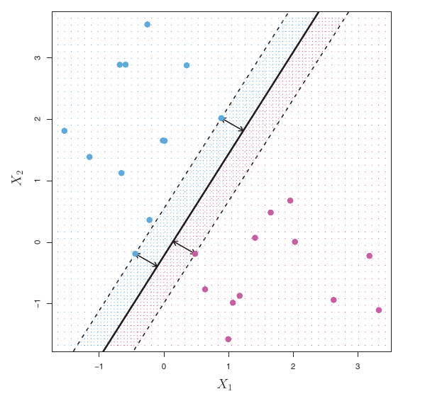
- The main idea consists in mapping the input space in a high-dimensional feature space ( generally a suitable Hilbert space) through nonlinear transformation to produce Optimal Separating Hyperplanes (OSH) that separates cases of different class label.
Support Vector Machine (SVM)
For simplicity, assume that the input data points are \(\mathbf{x}_i \in \mathbb{R}^p\) and \(y_i \in \{ -1, 1 \}\) are the class labels, with \(i = 1, \ldots, n\).
Intuitively, based on the training set, the SVM estimates a hyperplane that serves as a decision boundary, it is
\[
\langle \mathbf{w},\mathbf{x}_1 \rangle + b = w_1 x_{11} + w_2 x_{12} + \cdots + w_p x_{1p} + b = 0,
\]
where the weight vector \(\mathbf{w} \in \mathbb{R}^p\) and the bias \(b \in \mathbb{R}\).
- To predict the label of a new input vector \(\mathbf{x}_r\), the SVM uses the sign of the decision function:
\[
\hat{y}_r = \mathrm{sign}(\langle \mathbf{w},\mathbf{x}_r \rangle + b).
\]
Support Vector Machine (SVM)
- To find the optimal hyperplane, an optimization problem is formulated as follows:
\[\begin{align}
\label{EQ:SVM1}
\min_{ \mathbf{w} \in \mathbb{R}^p, b \in \mathbb{R}, \geq 0 }
f_{sv} = \dfrac{1}{2} \| \mathbf{w}\|_2^2 + C \mathbf{1}^\top \boldsymbol{\xi},
\end{align}\]
subject to the margin constraints \(y_i (\mathbf{w} \psi(\mathbf{x}_i) + b) \geq 1 − \xi_i\), \(\forall i\). Here \(\mathbf{1}\) is a vector of all 1’s. The Lagrange dual can be easily derived:
\[\begin{align}
\max_{ \boldsymbol{\alpha} } \mathbf{1}^\top \boldsymbol{\alpha} - \dfrac{1}{2} \boldsymbol{\alpha}^\top \left( K \circ \mathbf{y}\mathbf{y}^\top \right) \boldsymbol{\alpha}, \, \text{s.t.}\,0 \leq \boldsymbol{\alpha} \leq C, \mathbf{y}^\top \boldsymbol{\alpha} = 0,
\end{align}\]
here \(C\) is the trade-off parameter; \(K\) is the kernel matrix with \(K_{lh} = K(\mathbf{x}_l,\mathbf{x}_h)\); and \(\circ\) denotes element-wise matrix multiplication (Hadamard product).
Extreme Gradient Boosting (XGBoost)
- The XGBoost classifier is a decision-tree-based ensemble method that uses the decision tree concept associated with the Gradient Boosting structure.
- Therefore, this method is based on the boosting technique, which consists of re-sampling classifiers, with replacement, several times, however, the re-sampled data are constructed in such a way that they obtain learning from the classification performed in the previous sampling.
- To obtain the final result, after all re-sampling, a combination method weighted by the classification performance in each model is used.
Extreme Gradient Boosting (XGBoost)
- Consider a data set \(\mathcal{D} = \{(\mathbf{x}_i, y_i),i=1,\ldots,n\},\) with features \(\mathbf{x}_i\in \mathbb{R}^p\) and target variable \(y_i \in \mathbb{R}\). A predictive model based on tree ensemble can be described by
\[\begin{equation}
\widehat{y}_i = \sum^B_{b=1} f_b(\mathbf{x}_i), \ \ f_b\in \mathcal{F},
\end{equation}\]
where \(K\) is the total number of trees, \(f_b\) for \(b\)-th tree is a function in the functional space \(\mathcal{F}\), and \(\mathcal{F}\) is the the set of all possible regression trees (also known as CART).
- In the training, each of new-trained CART will try to complement the so-far residual.
Extreme Gradient Boosting (XGBoost)
- Objective function been optimized at \((t+1)\)-th CART is described: \[\begin{equation}\label{eq:loss}
\mathcal{L} = \sum_{i = 1}^n l( \widehat{y}_i^{(t)}, y_i ) + \sum_{b}\Omega( f_{b} ),
\end{equation}\] where \(l\) is a differentiable convex training loss function that measures the difference between the prediction \(\widehat{y}_i^{(t)}\) and the target \(y_i\) (ground truth) at step \(t.\) Here, the term \[\begin{equation}
\Omega(f) = \gamma T + \frac{1}{2} \lambda \|\mathbf{w}\|^2,
\end{equation}\] is the regularization fuction that helps to smooth the final learnt weights to avoid over-fitting. \(T\) are the number of leaves and \(\mathbf{w}\) is the score on leaf.
Naive Bayes
- The Naive Bayes (NB) classifier is a simple probabilistic classifier based on an application of Bayes’ theorem.
The classifier estimates a conditional probability density function of feature vectors by learning samples. Formally, assume a dataset \(\mathcal{D} = \{(\mathbf{x}_i, y_i), i=1,\ldots,n\},\) with \(\mathbf{x}_i\in \mathbb{R}^p\) and target variable \(y_i = c \in C\).
The NB predict the class label of the instance \(\mathbf{x}_r\) as follows:
\[\begin{equation} \label{key1}
\hat{c}_{NB}=\underset{c}{\mathrm{arg \, max}} P(c) \prod_{j=1}^p P(x_{rj}|c),
\end{equation}\]
where \(P(c)\) is the prior probability of class \(c\), and \(P(x_{rj} | c)\) is the conditional probability of the attribute value \(x_{rj}\) given the class \(c\).
Naive Bayes
\[
\hat{c}_{NB}=\underset{c}{\mathrm{arg \, max}} P(c) \prod_{j=1}^p P(x_{rj}|c),
\]
\[\begin{equation}\label{key2}
P(c)=\frac{\sum_{i=1}^n {\mathbb{I}(c_i,c)}} {n}
\end{equation}\]
\[\begin{equation}\label{key3}
P(x_{ij}|c)=\frac{\sum_{i=1}^n {\mathbb{I}(c_i,c)\mathbb{I}(x_{ij},A_{j})}}{\sum_{i=1}^n {\mathbb{I}(c_i,c)}},
\end{equation}\]
where \(A_j\) represents all the values of the \(j\)-th attribute in training instances, \(c_i\) denotes the correct class label for the \(i\)-th instance, and \(\mathbb{I}(a,b)\) is a indicator function, which takes the value 1 if \(a\) and \(b\) are identical and 0 otherwise.
Polarimetric Data multi-look
- Returning to the PolSAR data, we can consider that each pixel is generated by a linear combination of many contributions from different scattering mechanisms, such as surface scattering, volume scattering, and double-bounce scattering. So, by Central Limit Theorem, the return of each pixel can be modeled as a complex multivariate normal distribution.
- Thus, \(\mathbf{z}_i = (S_1^{(i)}\,S_2^{(i)}\,\cdots\,S_p^{(i)})^{\top} \, \in \mathbb{C}^{p}\), for \(i=1,\ldots,L\), follow a complex multivariate normal distribution with zero mean and covariance matrix \(\mathbf{\Sigma}\), that is, \(\mathbf{z} \sim N_{p}^{\mathbb{C}}(\mathbf{0},\mathbf{\Sigma})\) with probability density function:
\[f_{\mathbf{z}}(\dot{\mathbf{z}};\mathbf{\Sigma})= \dfrac{1}{\pi^{p}|\mathbf{\Sigma}|}\exp \left(-\dot{\mathbf{z}}^{*} \mathbf{\Sigma}^{-1} \dot{\mathbf{z}}\right),
\]
where \(|\cdot|\) is the determinant of a matrix or absolute value of a scalar, \((\cdot)^{*}\) is the conjugate transpose of a vector, and \(\mathbf{\Sigma}\) is the positive definite Hermitian covariance matrix that contains all necessary information to characterize the polarimetric return of the data under analysis.
Polarimetric Data multi-look
- The multi-look process is defined as \(\mathbf{Z} = L^{-1} \sum_{i=1}^{L}\mathbf{z}_i\mathbf{z}_i^{*}\) and, for \(\mathbf{z}_i \sim N_{p}^{\mathbb{C}}(\mathbf{0}, \mathbf{\Sigma})\), it follows a scaled complex Wishart distribution with probability density function given by:
\[
f_{\mathbf{Z}}(\dot{\mathbf{Z}};{\mathbf{\Sigma}},L) = \dfrac{L^{p^{L}}|\dot{\mathbf{Z}}|^{L-p}}{|\mathbf{\Sigma}|^{L}\Gamma_p(L)}\exp\left[-L\text{tr}(\mathbf{{\Sigma}}^{-1}\dot{\mathbf{Z}})\right],
\]
where \(\Gamma_p(L) = \pi^{p(p-1)/2}\prod_{i=0}^{p-1}\Gamma(L-i)\), \(L \geq p\), representing the multivariate gamma function, \(\Gamma(\cdot)\) is the gamma function, and \(\text{tr}(\cdot)\) is the trace operator.
- The WSCW distributio have two parameters:
- \(L\) is the number of looks, which controls the amount of speckle in the data;
- \(\mathbf{\Sigma}\) is the covariance matrix, which maps the dependence between the polarization channels.
Stochastic distances
Let \(\mathbf{X}\) and \(\mathbf{Y}\) be two random matrices defined in the common support \(\mathcal{Z}\) with densities \(f_{\mathbf{X}}(\dot{\mathbf{Z}};\boldsymbol{\theta}_1)\) and \(f_{\mathbf{Y}}(\dot{\mathbf{Z}};\boldsymbol{\theta}_2)\), respectively, where \(\boldsymbol{\theta}_1\) and \(\boldsymbol{\theta}_2\) are parameter vectors.
Then, a function is considered a stochastic distance, say \(d(\cdot,\cdot)\), between two random matrices if the following properties are satisfied:
\(d(\dot{\mathbf{X}},\dot{\mathbf{Y}}) \geq 0\) (non-negativity);
\(d(\dot{\mathbf{X}},\dot{\mathbf{Y}}) = 0 \Leftrightarrow \dot{\mathbf{X}} = \dot{\mathbf{Y}}\) (identity);
\(d(\dot{\mathbf{X}},\dot{\mathbf{Y}}) = d(\dot{\mathbf{Y}},\dot{\mathbf{X}})\) (symmetry);
The Kullback-Leibler classifier
- Let \(\mathbf{X}\) and \(\mathbf{Y}\) are two random matrices defined in the common support \(\mathcal{X}\) that have Wishart distributions, i.e., \(\mathbf{X} \sim \mathcal{W_p}^{\mathbb{C}} (L_1,\boldsymbol{\Sigma}_1)\) and \(\mathbf{Y} \sim \mathcal{W_p}^{\mathbb{C}} (L_2,\boldsymbol{\Sigma}_2)\) with densities \(f_{\boldsymbol{X}}(\boldsymbol{Z}';\boldsymbol{\theta}_1)\) and \(f_{\boldsymbol{Y}}(\boldsymbol{Z}';\boldsymbol{\theta}_2)\), respectively, where \(\boldsymbol{\theta}_1=(L_1,\boldsymbol{\Sigma}_1)\) and \(\boldsymbol{\theta}_2=(L_2,\boldsymbol{\Sigma}_2)\) are parameters. The Kullback-Leibler distance is defined by
\[\begin{align}%
d_\text{KL}(\mathbf{X},\mathbf{Y})=&\frac{L_1-L_2}{2}\bigg\{\log\frac{|\boldsymbol{\Sigma}_1|}{|\boldsymbol{\Sigma}_2|}-p\log\frac{L_1}{L_2}\nonumber +\psi_p^{(0)}(L_1)-\psi_p^{(0)}(L_2)\bigg\} \nonumber \\ &-\frac{p(L_1+L_2)}{2}
%&+(L_2-L_1)\displaystyle \sum_{i=1}^{m-1}\frac{i}{(L_1-i)(L_2-i)}\bigg\} \nonumber \\
+ \frac{\operatorname{tr}(L_2\boldsymbol{\Sigma}_2^{-1}\boldsymbol{\Sigma}_1+L_1\boldsymbol{\Sigma}_1^{-1}\boldsymbol{\Sigma}_2)}{2}.
\label{expreKL}
\end{align}\]
- In this study, \(L_1=L_2=L\) (generally \(L=4\)), and the before expression reduce to
The Kullback-Leibler classifier
\[\begin{equation}
d_{\text{KL}}(\boldsymbol{X},\boldsymbol{Y}) = L\bigg\{
\frac{\operatorname{tr}(\boldsymbol{\Sigma}_2^{-1}\boldsymbol{\Sigma}_1+\boldsymbol{\Sigma}_1^{-1}\boldsymbol{\Sigma}_2)}{2} - p\bigg\}.
\end{equation}\]
- In this way, a classification strategy use a supervised scheme based on stochastic distance between between pairs of complex Wishart distributions that model segments of PolSAR data on training samples which represent classes. The assignation of a class is given by the minimization of the stochastic distance \(d_{\text{KL}}\) in a segment, i.e.
\[
\hat{c}_{KL} = \underset{c}{\mathrm{arg min}} \ d_{\text{KL}}(\mathbf{X},\mathbf{Y}),
\]
- Kullback-Leibler distance has been used for PolSAR classification, with outstanding results, in deep neural networks as the main component of the loss function.
Experimental Setup
Actual PolSAR data
In this section, we describe the experiments carried out to validate our analysis of the selected classification methods.
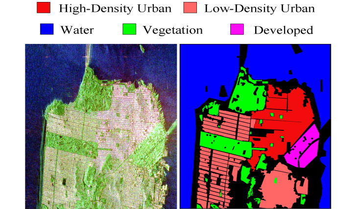
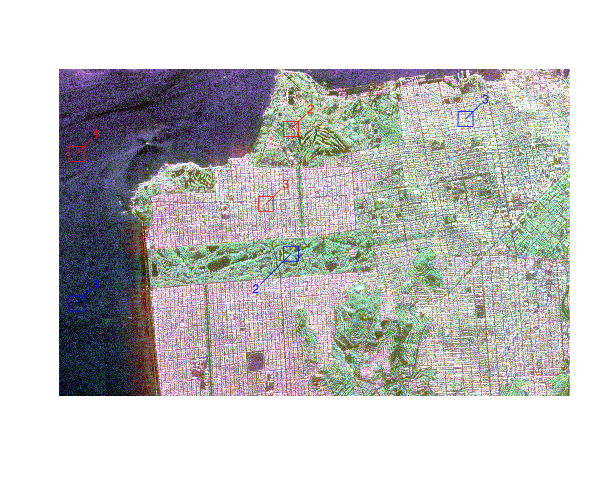
PolSAR data (\(Looks = 4\)) of size \(1600 \times 1200\) pixels acquired by the C-band RADARSAT-2 PolSAR system over the San Francisco area
![]()
Pauli-basis image of the RADARSAT-2 San Francisco data (left) and ground truth (right).
Experimental Setup
Evaluation criteria
Confusion Matrix:
\[
M = \begin{bmatrix}
n_{11} & \dots & n_{1c}\\
\vdots & \ddots & \vdots\\
n_{c1} & \dots& n_{cc}
\end{bmatrix}
\]
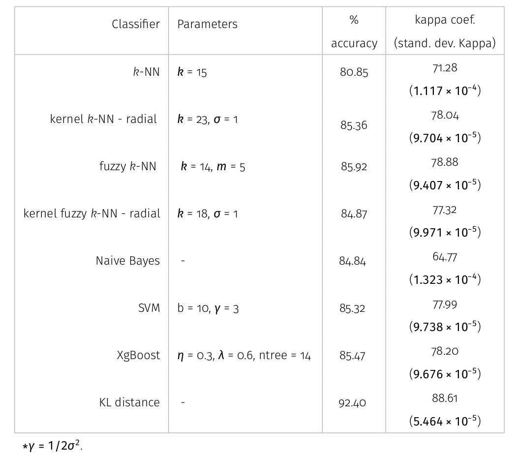
Accuracy and Kappa coefficient
\[\begin{equation}
AC={\sum^{c}_{i=1}n_{ii}}/N,
\end{equation}\]
\[\begin{equation}
\kappa={(Ac-P_{c})}/{(1-P_{c})},
\end{equation}\] where \(P_c= \sum_{i=1}^{c} (n_{i.}n_{.j})/N^2\). The ideal values for both indices are 1 (\(100\%\) in percentages).
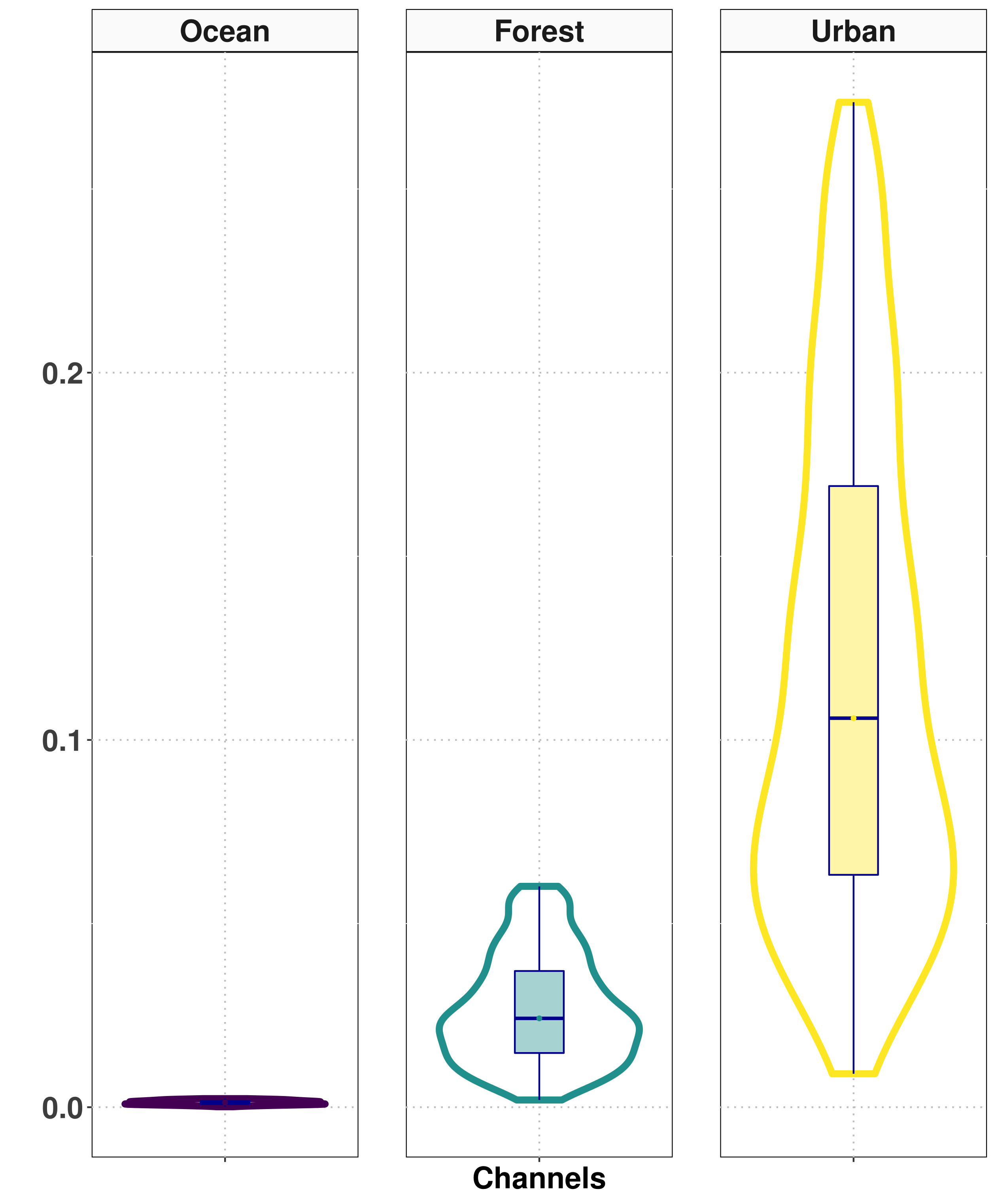
Experimental Setup
Selection of samples for training the classifiers
- The Ocean Area: Dimensions of 26×16 pixels for the training sample and 41×21 pixels for the test sample.
- The Forest: 23×16 pixels for the training sample and 41×21 pixels for the test sample.
- The Urban Area: 40×15 pixels for the training sample and 41×21 pixels for the test sample.
![]()
Experimental Setup
Selection of samples for training the classifiers
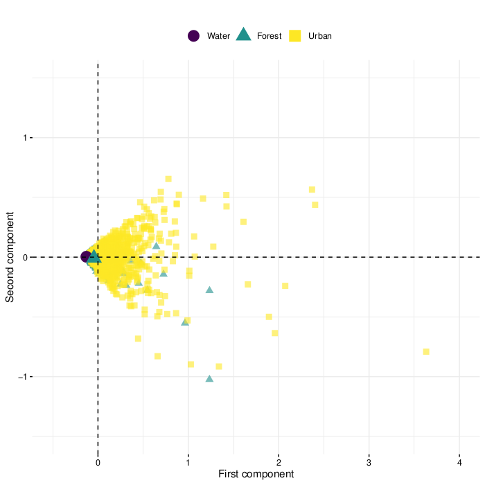
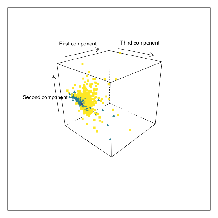
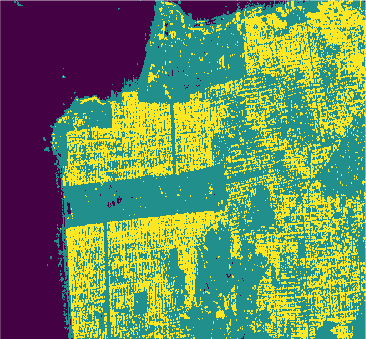
Results
![]()
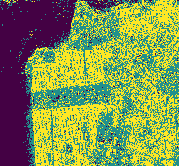
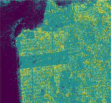
Results
Fuzzy k-NN
Fuzzy kernel k-NN
Conclusion
In this study we used eight classification algorithms, four based on -NN, one based on naive Bayes, one that uses Support Vector Machine (SVM), one produced by randomized decision tree and finally one based on stochastic distance. The latter exploits in a natural way the stochastic nature of the PolSAR data, that is, it is well-suited to this kind of remote sensing data.
The algorithms were used to classify the PolSAR data intensities of the regions of a well-known PolSAR dataset: the San Francisco Bay region.
All classifiers for San Francisco-USA image had a kappa coefficient above 80% and below 93%. It is clear the nowadays deep learning techniques show classification results with kappa \(\approx\) 1. However, at mentioned above, deep learning techniques require extensive training and results are difficult to reproduce.
- Additionally, it has been shown that there is room to improve their present capabilities (\(\approx 90\)) to keeping competitive to the new paradigms offered by deep learning methods.
References
ANFINSEN SN, DOULGERIS AP & ELTOFT T. 2009. Estimation of the equivalent number of looks in polarimetric synthetic aperture radar imagery. EEE Trans Geosci Remote Sens 47(11): 3795-3809.
BISHOP CM. 2006. Pattern Recognition and Machine Learning (Information Science and Statistics). 1st ed. Springer-Verlag, 738 p.
CINTRA RJ, FRERY AC & NASCIMENTO AD. 2013. Parametric and nonparametric tests for speckled imagery. Pattern Anal Appl 16(2): 141-161
FERREIRA JA, COÊLHO H & NASCIMENTO AD. 2021. A family of divergence-based classifiers for Polarimetric Synthetic Aperture Radar (PolSAR) imagery vector and matrix features. Int J Remote Sens 42(4): 1201-1229.
FRERY AC, NASCIMENTO ADC & CINTRA RJ. 2011. Information Theory and Image Understanding: An Application to Polarimetric SAR Imagery. Chil J Stat 2(2): 81-100.
LEE JS & POTTIER E. 2009. Polarimetric Radar Imaging From Basics to Applications. CRC Press.