Tópicos Especiais em Estatística Comp.
Redes Neurais fully conected (Totalmente Conectadas)
UFPE
Redes Neurais fully conected
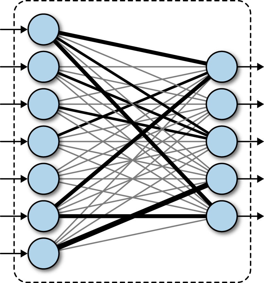
- Uma rede neural totalmente conectada, é um tipo de rede neural em que as camadas são totalmente conectadas, ou seja, cada nó ou neurônio de uma camada é conectada a todos os nós (neurônios) da camada seguinte.
Essa estrutura lembra algo a vocês?
MLP - Multilayer Perceptron
Redes Neurais fully conected
- Seja \(\mathbf{X} \in \mathbb{R}^{n \times p}\) a matriz de valores de entrada com \(n\) observações e \(p\) variáveis (features).

- Um MLP ou Rede Neural fully conected de uma camada oculta com \(h_{K}\) neurônios na camada oculta pode ser representada por uma matriz \(\mathbf{H} \in \mathbb{R}^{p \times h_K}\), em que \(\mathbf{H}\) também é conhecido como uma variável de camada oculta ou uma variável oculta.
Redes Neurais fully conected
em que \(\mathbf{H}\) é obtida como:
\[\mathbf{H} = \varphi (\mathbf{X} \mathbf{W}^{(1)} + \mathbf{b}^{(1)}),\]
onde \(\varphi(\cdot)\) é a função de ativação, \(\mathbf{W}^{(1)} \in \mathbb{R}^{p \times h_K}\) são os pesos da camada oculta e \(\mathbf{b}^{(1)} \in \mathbb{R}^{1 \times h_K}\) é o viés da camada oculta.
Como estamos em um MLP de camada única, a próxima camada é a camada de saída.
- A camada de \(\mathbf{O} \in \mathbb{R}^{h_K \times q}\), do MLP de uma camada oculta é calculada como:
\[\mathbf{O} = \varphi ( \mathbf{H}\mathbf{W}^{(2)} + \mathbf{b}^{(2)} ),\]
onde \(\mathbf{W}^{(2)} \in \mathbb{R}^{h_K \times q}\) são os pesos da camada de saída e \(\mathbf{b}^{(2)} \in \mathbb{R}^{1 \times q}\) é o viés da camada de saída, \(q\) é a dimensão de saída, por exemplo, em um problema de classificação é a quantidade de classes, em um problema de regressão \(q = 1\).
Redes Neurais fully conected
Um exemplo de MLP com uma camada oculta numericamente:
- Suponha que temos uma matriz de entrada \(\mathbf{X} \in \mathbb{R}^{3 \times 2}\) com 3 observações e 2 variáveis (features):
\[\mathbf{X} = \begin{bmatrix} 1 & 2 \\ 3 & 4 \\ 5 & 6 \end{bmatrix}\]
- Suponha que a camada oculta tenha 2 neurônios (\(h_K = 2\)), então os pesos da camada oculta \(\mathbf{W}^{(1)} \in \mathbb{R}^{2 \times 2}\) e o viés \(\mathbf{b}^{(1)} \in \mathbb{R}^{1 \times 2}\) são:
\[\mathbf{W}^{(1)} = \begin{bmatrix} 0.1 & 0.2 \\ 0.3 & 0.4 \end{bmatrix}, \quad \mathbf{b}^{(1)} = \begin{bmatrix} 0.5 & 0.6 \end{bmatrix}\]
Redes Neurais fully conected
- Calculamos a camada oculta \(\mathbf{H}\) usando a função de ativação ReLU: \[\mathbf{H} = \text{ReLU}(\mathbf{X} \mathbf{W}^{(1)} + \mathbf{b}^{(1)})\]
- Calculando \(\mathbf{X} \mathbf{W}^{(1)}\): \[\mathbf{X} \mathbf{W}^{(1)} = \begin{bmatrix} 1 & 2 \\ 3 & 4 \\ 5 & 6 \end{bmatrix} \begin{bmatrix} 0.1 & 0.2 \\ 0.3 & 0.4 \end{bmatrix} = \begin{bmatrix} 0.7 & 1.0 \\ 1.5 & 2.2 \\ 2.3 & 3.4 \end{bmatrix}\]
- Adicionando o viés \(\mathbf{b}^{(1)}\): \[\mathbf{X} \mathbf{W}^{(1)} + \mathbf{b}^{(1)} = \begin{bmatrix} 0.7 & 1.0 \\ 1.5 & 2.2 \\ 2.3 & 3.4 \end{bmatrix} + \begin{bmatrix} 0.5 & 0.6 \end{bmatrix} = \begin{bmatrix} 1.2 & 1.6 \\ 2.0 & 2.8 \\ 2.8 & 4.0 \end{bmatrix}\]
Redes Neurais fully conected
Aplicando a função ReLU: \[\mathbf{H} = \text{ReLU}\left(\begin{bmatrix} 1.2 & 1.6 \\ 2.0 & 2.8 \\ 2.8 & 4.0 \end{bmatrix}\right) = \begin{bmatrix} 1.2 & 1.6 \\ 2.0 & 2.8 \\ 2.8 & 4.0 \end{bmatrix}\]
Suponha que a camada de saída tenha 1 neurônio (\(q = 1\)), então os pesos da camada de saída \(\mathbf{W}^{(2)} \in \mathbb{R}^{2 \times 1}\) e o viés \(\mathbf{b}^{(2)} \in \mathbb{R}^{1 \times 1}\) são: \[\mathbf{W}^{(2)} = \begin{bmatrix} 0.5 \\ 0.6 \end{bmatrix}, \quad \mathbf{b}^{(2)} = \begin{bmatrix} 0.7 \end{bmatrix}\]
Redes Neurais fully conected
- Calculamos a saída \(\mathbf{O}\): \[\mathbf{O} = \text{Linear} ( \mathbf{H}\mathbf{W}^{(2)} + \mathbf{b}^{(2)} )\]
- Calculando \(\mathbf{H}\mathbf{W}^{(2)}\): \[\mathbf{H}\mathbf{W}^{(2)} = \begin{bmatrix} 1.2 & 1.6 \\ 2.0 & 2.8 \\ 2.8 & 4.0 \end{bmatrix} \begin{bmatrix} 0.5 \\ 0.6 \end{bmatrix} = \begin{bmatrix} 1.62 \\ 2.68 \\ 3.74 \end{bmatrix}\]
Redes Neurais fully conected
- Adicionando o viés \(\mathbf{b}^{(2)}\): \[\mathbf{O} = \begin{bmatrix} 1.62 \\ 2.68 \\ 3.74 \end{bmatrix} + \begin{bmatrix} 0.7 \end{bmatrix} = \begin{bmatrix} 2.32 \\ 3.38 \\ 4.44 \end{bmatrix}\]
- Portanto, a saída final do MLP com uma camada oculta é: \[\mathbf{O} = \begin{bmatrix} 2.32 \\ 3.38 \\ 4.44 \end{bmatrix}\]
Redes Neurais fully conected
- Para construir MLPs mais gerais, podemos continuar empilhando tais camadas ocultas, como por exemplo:
\[\mathbf{H}^{(1)} = \varphi_1(\mathbf{X} \mathbf{W}^{(1)} + \mathbf{b}^{(1)})\]
\[\mathbf{H}^{(2)} = \varphi_2(\mathbf{H}^{(1)} \mathbf{W}^{(2)} + \mathbf{b}^{(2)})\]
\[\vdots\]
\[\mathbf{O} = \varphi_g(\mathbf{H}^{(d)} \mathbf{W}^{(d)} + \mathbf{b}^{(d)})\]
em que \(d\) é a última camada oculta, anterior à camada de saída, \(\mathbf{W}^{(i)}\) e \(\mathbf{b}^{(i)}\) são os pesos e o viés da \(i\)-ésima camada oculta, e \(\varphi_i(\cdot)\) é a função de ativação da \(i\)-ésima camada oculta.
Redes Neurais fully conected
- Essas redes neurais mais complexas são chamadas de MLPs de múltiplas camadas ou redes neurais fully conected profundas.
- Assim, a diferença entre uma rede neural fully conected e uma MLP (Multilayer Perceptron) é apenas questão de nomenclatura, pois uma MLP também é uma rede neural fully conected.
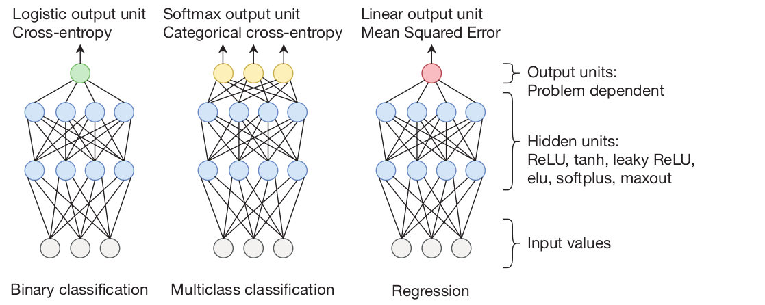
Podemos ter em geral 3 tipos de saídas de uma rede neural fully conected:
Classificação Binária: utiliza-se a função sigmóide como função de ativação na última camada e a função de perda entropia cruzada.
Classificação Multiclasse: utiliza-se a função softmax como função de ativação na última camada e a função de perda entropia cruzada.
Regressão: utiliza-se a função identidade como função de ativação na última camada e a função de perda erro quadrático médio (MSE).
Redes Neurais fully conected
Redes Neurais fully conected
Vamos executar cada um deles no python
Referências para serem utilizadas
BRAGA, A. P.; CARVALHO, A.; LUDEMIR, T. Redes Neurais Artificiais: Teoria e Aplicações. .: [s.n.], 2000.
HOPFWELD, J. J. Neural networks and physical systems with emergent collective computational abilities. Proc. NatL Acad. Sci., v. 79, p. 2554–2558, 1982.
LUDWIG, O.; MONTGOMERY, E. Redes Neurais - Fundamentos e Aplicações com Programas em C. .: Ciência Moderna, 2007.
MINSKY, M.; PAPERT, S. Perceptrons: an introduction to computationational geometry. [S.l.]: MIT Press, 1969.
PINHEIRO, C. A. R. Inteligência Analítica: Mineração de Dados e Descoberta de Conhecimento. .: [s.n.], 2008.
RICH, E.; KNIGHT, K. Inteligência Artificial. .: [s.n.], 1993.
ROSENBLATT, F. Principles of Neurodynamics: Perceptrons and Theory of Brain Mechanisms. .: Washigton, DC, 1962.
OBRIGADO!
Slide produzido com quarto
Tópicos Especiais em Estatística Comp. - Prof. Jodavid Ferreira