Statistical Machine Learning

Parametric Methods for Regression

Prof. Jodavid Ferreira

UFPE

Notation

---

• \(X\) or \(Y\)
• \(x\) or \(y\)
• \(\mathbf{x}\) or \(\mathbf{y}\)
• \(\dot{\mathbf{x}}\) or \(\dot{\mathbf{y}}\)
• \(\mathbf{X}\) or \(\mathbf{Y}\)
• \(\dot{\mathbf{X}}\) or \(\dot{\mathbf{Y}}\)

• \(p\)
• \(n\)
• \(i\)
• \(j\)
• \(k\)

represent random variables (r.v.);

represent realizations of random variables;

represent random vectors;

represent realizations of random vectors;

represent random matrices;

represent realizations of random matrices;

dimension of features, variables, parameters

sample size

\(i\)-th observation, instance (e.g., \(i=1, ..., n\))

\(j\)-th feature, variable, parameter (e.g., \(j=1, ..., p\))

number of folds in k-fold CV

Motivation:

Evaluating Model Performance

---

• In machine learning, we build models to make predictions on new, unseen data.

• How do we know how well our model will perform on this unseen data?

• We need ways to estimate the validation error: the average error when applying our model to new observations. We often denote the true regression function as \(f(x) = \mathbb{E}[Y|X=x]\) and our estimate as \(\hat{f}(x)\). The risk is \(R(\hat{f}) = \mathbb{E}[(Y - \hat{f}(X))^2]\).

• Simply using the training error (error on the data used to build the model) is often misleadingly optimistic. Models can overfit the training data.

Parametric Methods

---

• Assume the regression function \(f(x)\) can be parameterized by a finite number of parameters.

• Focus: Linear Regression models.

• Much of this might be review, but perhaps from a different perspective.

• We model the prediction function \(\hat{f}(x)\) using a linear form:

  \[ \hat{f}(\mathbf{x}) = \boldsymbol{\beta}^\top \mathbf{x} = \beta_0 + \beta_1 x_1 + \dots + \beta_p x_p \]

• \(\boldsymbol{\beta} = (\beta_0, \beta_1, \dots, \beta_p)^\top\) is the vector of parameters.

• \(\mathbf{x} = (1, x_1, \dots, x_p)^\top\) is the vector of predictors (features).

Predictor Variables (Features)

---

\[ \hat{f}(\mathbf{x}) = \boldsymbol{\beta}^\top \mathbf{x} = \beta_0 + \beta_1 x_1 + \dots + \beta_p x_p \]

• The components \(x_j\) (\(j=1, \dots, p\)) are not necessarily the original measured variables.
• They can be transformations or combinations of original variables.
  • Polynomial terms: \(x_j^2, x_j^3, \dots\)
  • Interaction terms: \(x_j x_k\)
  • Other functions: \(\log(x_j)\), \(\sqrt{x_j}\), etc.
• The model is linear in the parameters \(\boldsymbol{\beta}\).

Estimating Coefficient

Ordinary Least Squares (OLS)

---

• Given a training dataset \((\dot{\mathbf{x}}_1, y_1), \dots, (\dot{\mathbf{x}}_n, y_n)\), where \(\dot{\mathbf{x}}_i = (1,x_{i1}, \dots, x_{ip})^\top\).
• Goal: Find the parameter vector \(\boldsymbol{\beta}\) that minimizes the Residual Sum of Squares (RSS):

\[\hat{\boldsymbol{\beta}}_{OLS} = \arg \min_{\boldsymbol{\beta}} \sum_{i=1}^n (y_i - \boldsymbol{\beta}^\top \dot{\mathbf{x}}_i)^2\]

• This is also often written as minimizing \(||\dot{\mathbf{y}} - \dot{\mathbf{X}} \boldsymbol{\beta}||^2\).

OLS Solution

---

• Let \(\dot{\mathbf{y}} = (y_1, \dots, y_n)^\top\) be the vector of responses.

• Let \(\dot{\mathbf{X}}\) be the \(n \times (p+1)\) design matrix:

  \[ \dot{\mathbf{X}} = \begin{pmatrix} 1 & x_{11} & \dots & x_{1p} \\ 1 & x_{21} & \dots & x_{2p} \\ \vdots & \vdots & \ddots & \vdots \\ 1 & x_{n1} & \dots & x_{np} \end{pmatrix} \]

• The OLS solution is given by the normal equations: \((\dot{\mathbf{X}}^\top \dot{\mathbf{X}}) \hat{\boldsymbol{\beta}} = \dot{\mathbf{X}}^\top \dot{\mathbf{y}}\).

• If \((\dot{\mathbf{X}}^\top \dot{\mathbf{X}})\) is invertible (requires \(n \ge p+1\) and full column rank):

  \[ \hat{\boldsymbol{\beta}}_{OLS} = (\dot{\mathbf{X}}^\top \dot{\mathbf{X}})^{-1} \dot{\mathbf{X}}^\top \dot{\mathbf{y}} \]

OLS Prediction Function

---

• Once we have the estimated coefficients \(\hat{\boldsymbol{\beta}}_{OLS}\), the prediction function is:

  \[ \hat{f}_{OLS}(\mathbf{x}) = \hat{\boldsymbol{\beta}}_{OLS}^\top \mathbf{x} \]

• Where \(\mathbf{x} = (1, x_1, \dots, x_p)^\top\) is a new input vector.

In R:

• Example: Predict response using predictor1 and predictor2 from my_dataframe.

# Criar uma base de dados com 5.000 valores
set.seed(123) # Para garantir reprodutibilidade dos resultados

n <- 5000 # Número de observações

predictor1 <- runif(n, min = 0, max = 100) # Valores aleatórios entre 0 e 100
predictor2 <- rnorm(n, mean = 50, sd = 15) # Valores aleatórios com média 50 e desvio padrão 15

# Gerar a resposta com base em uma relação linear com os preditores e algum ruído
response <- 10 + 2 * predictor1 - 0.5 * predictor2 + rnorm(n, mean = 0, sd = 10)

# Criar o dataframe
my_dataframe <- data.frame(
  response = response,
  predictor1 = predictor1,
  predictor2 = predictor2
)

# Exibir as primeiras linhas do dataframe e sua dimensão
head(my_dataframe)
dim(my_dataframe)

OLS in R

---

• The lm() function in R fits linear models using OLS.

# Carregar pacotes necessários
library(tidymodels)

# Certificar que 'my_dataframe' existe (criado no passo anterior)
# Se não existir, execute o código para criar a base com 5.000 valores

# 1. Data Splitting
set.seed(456) # Para reprodutibilidade da divisão dos dados
data_split <- initial_split(my_dataframe, prop = 0.8) # 80% para treino, 20% para teste
train_data <- training(data_split)
validation_data <- testing(data_split)


# 2. Cross-Validation
set.seed(789) # Para reprodutibilidade da criação das folds de validação cruzada
folds <- vfold_cv(train_data, v = 10) # Criar 10 folds de validação cruzada

# 3. Especificação do Modelo (já definido anteriormente)
ols_spec <- linear_reg() |> 
  set_engine("lm")

# 4. Workflow (combina a especificação do modelo e a fórmula)
ols_workflow <- workflow() |> 
  add_model(ols_spec) |> 
  add_formula(response ~ predictor1 + predictor2)

# 5. Ajustar o modelo usando validação cruzada
cv_results <- fit_resamples(
  ols_workflow,
  resamples = folds,
  metrics = metric_set(rmse, rsq, mae) # Métricas para avaliar o desempenho
)

# Exibir os resultados da validação cruzada
collect_metrics(cv_results,summarize = TRUE)
collect_metrics(cv_results,summarize = FALSE)

# 6. Ajustar o modelo final aos dados de treino
final_fit <- fit(ols_workflow, data = train_data)

# 7. Fazer previsões nos dados de validacao
predictions <- predict(final_fit, new_data = validation_data)

# 8. Avaliar o modelo nos dados de validation
validation_results <- validation_data |> 
  bind_cols(predictions) |> 
  metrics(truth = response, estimate = .pred)

print("Resultados da Validação Cruzada:")
print(collect_metrics(cv_results))

print("\nResultados no Conjunto de Validação:")
print(validation_results)

plot(predictions$.pred,validation_data$response)

The Linearity Assumption

---

• A core assumption often made in introductory treatments is that the true relationship \(f(x) = \mathbb{E}[Y|X=x]\) is actually linear. \[ f(\mathbf{x}) = \boldsymbol{\beta}^\top \mathbf{x} \quad \text{(for some true } \boldsymbol{\beta})\]

• In practice, this is a very strong assumption and often unrealistic.

Question: What does OLS estimate if the true relationship is not linear?

OLS and the Best Linear Predictor

---

• Even if \(f(x)\) is non-linear, we can still ask: What is the best linear approximation to \(f(x)\) in terms of minimizing expected squared error?

• Define the best linear predictor \(\boldsymbol{\beta}_*\) as the vector minimizing the expected prediction error over the data distribution¹:

  \[ \boldsymbol{\beta}_* = \arg \min_{\boldsymbol{\beta}} \mathbb{E}[(Y - \boldsymbol{\beta}^\top \mathbf{X})^2]\]

• \(\boldsymbol{\beta}_*\) represents the coefficients of the linear function \(g_{\boldsymbol{\beta}_*}(x) = \boldsymbol{\beta}_*^\top \mathbf{x}\) that is closest to the true response \(Y\) on average.²

1. (Note: Expectation is over the joint distribution of \((X, Y)\))

2. (Note: Kept \(g_{\boldsymbol{\beta}_*}\) as it refers to the theoretical best linear function, not the sample estimate \(\hat{f}\))

Theorem

Asymptotic Convergence of the OLS Estimator

---

• In Machine Learning, we build models (\(\hat{f}\)) from finite data samples.

• Fundamental Question: How does our model behave as we get more data (\(n \to \infty\))?
  • Does our estimated parameter (\(\hat{\boldsymbol{\beta}}\)) approach some “true” or “best” value?
  • Does the performance (e.g., prediction error) of our learned model stabilize or improve?

• Asymptotic Theory: Provides guarantees about the long-run behavior of our estimators and models.

• Today’s Focus: The asymptotic behavior of the Ordinary Least Squares (OLS) estimator.

Theorem

Asymptotic Convergence of the OLS Estimator

---

1. Best Linear Predictor (BLP) Parameters (\(\boldsymbol{\beta}_*\)):
   • The parameter vector \(\boldsymbol{\beta}_* \in \mathbb{R}^p\) that defines the best possible linear function \(\hat{f}_{\boldsymbol{\beta}_*}(\mathbf{x}) = \mathbf{x}^\top \boldsymbol{\beta}_*\) for predicting \(Y\) from \(\mathbf{X}\) (in terms of expected squared error).
   • \(\boldsymbol{\beta}_* = \arg \min_{\boldsymbol{\beta} \in \mathbb{R}^p} \mathbb{E}[(Y - \boldsymbol{\beta}^\top \mathbf{X})^2]\)
   • Derived as: \(\boldsymbol{\beta}_* = (\mathbb{E}[\mathbf{X}\mathbf{X}^\top])^{-1} \mathbb{E}[Y\mathbf{X}] = \Sigma^{-1} \boldsymbol{\alpha}\) (Population quantities!)

2. Ordinary Least Squares (OLS) Estimator (\(\hat{\boldsymbol{\beta}}_{OLS}\)):
   • The parameter vector \(\hat{\boldsymbol{\beta}}_{OLS} \in \mathbb{R}^p\) calculated from a sample \(\{(y_i, \mathbf{x}_i)\}_{i=1}^n\) to minimize the sum of squared residuals.
   • \(\hat{\boldsymbol{\beta}}_{OLS} = \arg \min_{\boldsymbol{\beta} \in \mathbb{R}^p} \sum_{i=1}^n (y_i - \boldsymbol{\beta}^\top \mathbf{x}_i)^2\)
   • Calculated as: \(\hat{\boldsymbol{\beta}}_{OLS} = (\sum_{i=1}^n \mathbf{x}_i \mathbf{x}_i^\top)^{-1} (\sum_{i=1}^n y_i \mathbf{x}_i) = \hat{\Sigma}_n^{-1} \hat{\boldsymbol{\alpha}}_n\) (Sample quantities!)

Theorem

Asymptotic Convergence of the OLS Estimator

---

• Assumption:
  • The population covariance matrix \(\Sigma = \mathbb{E}[\mathbf{X}\mathbf{X}^\top]\) exists and is invertible (no multicollinearity in the population).

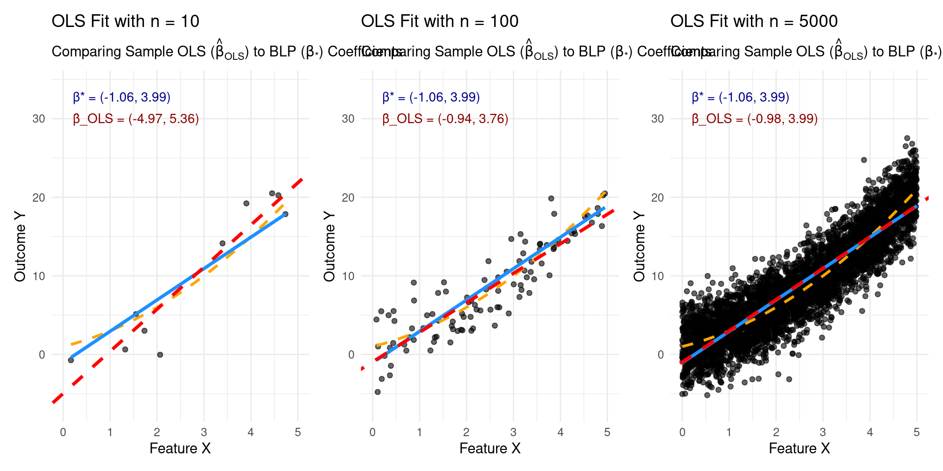
• Conclusion 1 (Parameter Convergence):
  • As the sample size \(n \to \infty\), the OLS estimator \(\hat{\boldsymbol{\beta}}_{OLS}\) converges in probability to the best linear predictor parameter vector \(\boldsymbol{\beta}_*\). \[\hat{\boldsymbol{\beta}}_{OLS} \xrightarrow{P} \boldsymbol{\beta}_*\]

What Does \(\hat{\boldsymbol{\beta}}_{OLS} \xrightarrow{P} \boldsymbol{\beta}_*\) Mean?

Theorem

Asymptotic Convergence of the OLS Estimator

---

What Does \(\hat{\boldsymbol{\beta}}_{OLS} \xrightarrow{P} \boldsymbol{\beta}_*\) Mean?

• It’s a statement about the behavior of the estimator \(\hat{\boldsymbol{\beta}}_{OLS}\) (which is a random vector, as it depends on the sample) as \(n\) grows.
• Informally: With enough data, the OLS estimate \(\hat{\boldsymbol{\beta}}_{OLS}\) is very likely to be very close to the target value \(\boldsymbol{\beta}_*\).
• Formally: For any small tolerance \(\epsilon > 0\), the probability that the distance between \(\hat{\boldsymbol{\beta}}_{OLS}\) and \(\boldsymbol{\beta}_*\) is larger than \(\epsilon\) goes to zero as \(n \to \infty\). \[ P(||\hat{\boldsymbol{\beta}}_{OLS} - \boldsymbol{\beta}_*|| > \epsilon) \to 0 \quad \text{as} \quad n \to \infty \]
• This property is called Consistency. \(\hat{\boldsymbol{\beta}}_{OLS}\) is a consistent estimator of \(\boldsymbol{\beta}_*\).

Theorem

Asymptotic Convergence of the OLS Estimator

---

• Recall:
  • \(\hat{f}_{OLS}(\mathbf{x}) = \mathbf{x}^\top \hat{\boldsymbol{\beta}}_{OLS}\) (Our estimated prediction function)
  • \(\hat{f}_{\boldsymbol{\beta}_*}(\mathbf{x}) = \mathbf{x}^\top \boldsymbol{\beta}_*\) (The best possible linear prediction function)
  • Risk \(R(h) = \mathbb{E}[(Y - h(\mathbf{X}))^2]\) (Expected squared prediction error)

• Conclusion 2 (Risk Convergence):
  • As the sample size \(n \to \infty\), the risk of the OLS predictor converges in probability to the risk of the best linear predictor. \[R(\hat{f}_{OLS}) \xrightarrow{P} R(\hat{f}_{\boldsymbol{\beta}_*})\]

What Does \(R(\hat{f}_{OLS}) \xrightarrow{P} R(\hat{f}_{\boldsymbol{\beta}_*})\) Mean?

Theorem

Asymptotic Convergence of the OLS Estimator

---

What Does \(R(\hat{f}_{OLS}) \xrightarrow{P} R(\hat{f}_{\boldsymbol{\beta}_*})\) Mean?

• The expected performance of the model we learned using OLS (\(\hat{f}_{OLS}\)) approaches the best possible expected performance we could ever get using any linear model (\(\hat{f}_{\boldsymbol{\beta}_*}\)).
• In Practice: As we train our OLS model on more and more data, its generalization error (how well it performs on unseen data, on average) approaches the theoretical minimum error achievable if we restrict ourselves to linear models.
• It tells us that OLS, given enough data, finds the optimally performing linear model.

Theorem

Asymptotic Convergence of the OLS Estimator

---

How Does OLS Converge? (Proof Intuition)

• Goal: Show \(\hat{\boldsymbol{\beta}}_{OLS} \to \boldsymbol{\beta}_*\) as \(n \to \infty\).
• Recall:
  • Target: \(\boldsymbol{\beta}_* = \Sigma^{-1} \boldsymbol{\alpha} = (\mathbb{E}[\mathbf{X}\mathbf{X}^\top])^{-1} \mathbb{E}[Y\mathbf{X}]\) (Population Level)
  • Estimator: \(\hat{\boldsymbol{\beta}}_{OLS} = \hat{\Sigma}_n^{-1} \hat{\boldsymbol{\alpha}}_n = (\frac{1}{n}\sum_{i=1}^n \mathbf{x}_i \mathbf{x}_i^\top)^{-1} (\frac{1}{n}\sum_{i=1}^n y_i \mathbf{x}_i)\) (Sample Level)
• The Bridge: We need tools to connect the sample averages (\(\hat{\Sigma}_n, \hat{\boldsymbol{\alpha}}_n\)) to the population expectations (\(\Sigma, \boldsymbol{\alpha}\)).
• Key Ingredients:
  1. Law of Large Numbers (LLN): Sample averages converge to expectations.
  2. Continuous Mapping Theorem (CMT) / Slutsky’s Theorem: Convergence carries through continuous functions (like matrix inversion and multiplication).

Theorem

Asymptotic Convergence of the OLS Estimator

---

Connecting Sample to Population: The LLN

• The Law of Large Numbers is the workhorse here.
• Assuming our data points \((y_i, \mathbf{x}_i)\) are i.i.d. and relevant expectations exist:
  • The sample covariance matrix converges to the population covariance matrix: \[ \hat{\Sigma}_n = \frac{1}{n}\sum_{i=1}^n \mathbf{x}_i \mathbf{x}_i^\top \xrightarrow{P} \mathbb{E}[\mathbf{X}\mathbf{X}^\top] = \Sigma \]
  • The sample cross-product vector converges to the population cross-product vector: \[ \hat{\boldsymbol{\alpha}}_n = \frac{1}{n}\sum_{i=1}^n y_i \mathbf{x}_i \xrightarrow{P} \mathbb{E}[Y\mathbf{X}] = \boldsymbol{\alpha} \]

Theorem

Asymptotic Convergence of the OLS Estimator

---

• Continuous Mapping Theorem / Slutsky’s Theorem: If \(Z_n \xrightarrow{P} Z\) and \(g\) is a continuous function, then \(g(Z_n) \xrightarrow{P} g(Z)\).
  • Matrix inversion is continuous (where the matrix is invertible). Since \(\Sigma\) is invertible (by assumption) and \(\hat{\Sigma}_n \to \Sigma\), then: \(\hat{\Sigma}_n^{-1} \xrightarrow{P} \Sigma^{-1}\)
  • Matrix multiplication is continuous. Applying the theorem (specifically Slutsky’s for products): \[ \hat{\boldsymbol{\beta}}_{OLS} = \underbrace{\hat{\Sigma}_n^{-1}}_{\xrightarrow{P} \Sigma^{-1}} \underbrace{\hat{\boldsymbol{\alpha}}_n}_{\xrightarrow{P} \boldsymbol{\alpha}} \xrightarrow{P} \Sigma^{-1} \boldsymbol{\alpha} = \boldsymbol{\beta}_* \]

• Done! \(\hat{\boldsymbol{\beta}}_{OLS}\) converges in probability to \(\boldsymbol{\beta}_*\).

Target is Best Linear Fit

OLS Finds the Best Linear Approximation

---

• Key Insight: OLS converges to \(\boldsymbol{\beta}_*\), the parameters of the Best Linear Predictor.

• It does not necessarily converge to parameters related to the true underlying function \(f(\mathbf{x})\) if \(f(\mathbf{x})\) is non-linear!
• Example: If \(Y = X^2 + \epsilon\), OLS will still fit the best line through the parabola, not recover the \(X^2\) relationship.

• Takeaway: OLS finds the optimal linear summary of the relationship between \(\mathbf{X}\) and \(Y\).

Target is Best Linear Fit

OLS is a Consistent Estimator (for \(\boldsymbol{\beta}_*\) )

---

• The result \(\hat{\boldsymbol{\beta}}_{OLS} \xrightarrow{P} \boldsymbol{\beta}_*\) means OLS is consistent.

• Practical Meaning: As you feed OLS more data, you can be increasingly confident that your estimated coefficients \(\hat{\boldsymbol{\beta}}_{OLS}\) are getting closer to the parameters \(\boldsymbol{\beta}_*\) of that best linear approximation.

Justification for Use

Why Use Linear Regression Even if Reality Isn’t Linear?

---

• Theorem provides a strong justification:
  • If your goal is simply to find a good linear approximation or a simple baseline model, OLS is asymptotically guaranteed to find the best one (in MSE sense).
• Linear models are:
  • Interpretable
  • Computationally cheap
  • Well-understood
• OLS gives us the optimal way to fit such a model, even under misspecification (i.e., when the true relationship isn’t linear).

Justification for Use

Why Use Linear Regression Even if Reality Isn’t Linear?

---

\[y = f(\mathbf{x}) = 1.0 + 2.0x_1 + 0.5x_1^2 + \epsilon,\]

where \(x \sim U[0,5]\) and \(\epsilon \sim \mathcal{N}(0,2.5)\)

Quality of Approximation

Limitation: Best Linear Fit != Good Overall Fit

---

• Theorem guarantees convergence to the best linear predictor \(\hat{f}_{\boldsymbol{\beta}_*}\), and \(R(\hat{f}_{OLS}) \to R(\hat{f}_{\boldsymbol{\beta}_*})\).

• BUT: The risk of the best linear predictor, \(R(g_{\boldsymbol{\beta}_*})\), might still be very high!

• If the true relationship \(f(\mathbf{x})\) is highly non-linear, the gap between \(R(f)\) and \(R(\hat{f}_{\boldsymbol{\beta}_*})\) can be large. This gap is the approximation error due to using a linear model.

• ML Takeaway: Just because OLS converges doesn’t mean linear regression is sufficient for your task. If \(R(\hat{f}_{\boldsymbol{\beta}_*})\) is high, you need more complex, non-linear models to get better performance.

Limitations of OLS

---

• High Variance / Overfitting: When the number of predictors \(p\) is large relative to the sample size \(n\), OLS coefficients can have high variance. The model fits the training data noise, leading to poor performance on new data (high validation error).

• Non-Invertibility: If \(p+1 > n\), the matrix \(\dot{\mathbf{X}}^\top \dot{\mathbf{X}}\) is singular (not invertible). The OLS estimator \(\hat{\boldsymbol{\beta}}_{OLS}\) is not uniquely defined.

• Multicollinearity: If predictors are highly correlated, \(\dot{\mathbf{X}}^\top \dot{\mathbf{X}}\) is ill-conditioned (near singular), leading to unstable coefficients with large standard errors.

• These issues become particularly prominent in high-dimensional settings.

---

High-Dimensional Data

---

High-Dimensional Data

---

• Modern datasets often have a large number of features/predictors (\(p\)).
  • Genomics: \(p\) (genes) > \(n\) (samples)
  • Text analysis: \(p\) (words/terms) can be very large
  • Finance: \(p\) (potential economic indicators)

• When \(p\) is large, OLS often performs poorly due to high variance or may not even be computable.

• We need methods that can handle high dimensions effectively.

Parametric Methods

in High Dimensions

---

• Problem: OLS has poor performance (low predictive power due to overfitting/high variance) when \(p\) is large.

• Goal: Find estimators that perform better in high dimensions.

• General Strategy: Introduce constraints or penalties to the estimation process to reduce variance, potentially at the cost of introducing some bias (Bias-Variance Trade-off).

Bias-Variance Trade-off Recap

---

• Expected Prediction Error (Risk) at a point \(x_0\):

  \[\mathbb{E}[(Y - \hat{f}(x_0))^2 | X=x_0] = \underbrace{(\mathbb{E}[\hat{f}(x_0)] - f(x_0))^2}_{\text{Squared Bias}} + \underbrace{Var(\hat{f}(x_0))}_{\text{Variance}} + \underbrace{Var(\epsilon)}_{\text{Irreducible Error}}\]

• OLS (Low Dimension): Typically low bias (if model is correct or \(\boldsymbol{\beta}_*\) is good approx.), variance depends on \(n, p, \sigma^2\).

• OLS (High Dimension): Low bias (for \(\boldsymbol{\beta}_*\)), but potentially huge variance.

• High-Dim Goal: Reduce variance significantly, even if bias increases slightly, to achieve lower overall expected error.

Best Subset Selection

---

• Idea: Assume only a subset of predictors are truly related to the response. Find the subset that yields the best model.

• Explicitly sets coefficients of unused predictors to zero.

• Formulation: For each possible subset size \(k \in \{0, 1, \dots, p\}\), find the subset of \(k\) variables that minimizes RSS. Then choose the best \(k\) using a criterion like AIC, BIC, or Cross-Validation.

Best Subset Selection

Penalized View

---

• Equivalent Formulation: Find \(\boldsymbol{\beta}\) to minimize:

  \[ \sum_{i=1}^n (y_i - \boldsymbol{\beta}^\top \dot{\mathbf{x}}_i)^2 + \lambda ||\boldsymbol{\beta}||_0 \]

  where \(||\boldsymbol{\beta}||_0 = \sum_{j=1}^p I(\beta_j \neq 0)\) is the “L0 norm” (counts non-zero coefficients)¹.

• The penalty parameter \(\lambda\) controls the number of non-zero coefficients. Larger \(\lambda\) encourages sparser models (fewer predictors).

1. Note: Intercept \(\beta_0\) is usually not penalized.

Best Subset Selection

Connection to AIC

---

• If the errors \(\epsilon_i\) are \(N(0, \sigma^2)\), minimizing the Akaike Information Criterion (AIC) is asymptotically equivalent to choosing the penalty \(\lambda \approx 2\sigma^2\) in the L0-penalized formulation. \[ AIC = -2 \log(\text{Maximized Likelihood}) + 2 \times (\text{# parameters}) \] \[ AIC \propto \frac{1}{n} RSS + \frac{2\sigma^2}{n} \times (\text{# non-zero betas}) \]
• So, finding the solution to the L0-penalized problem for \(\lambda = 2\sigma^2\) involves:
  1. Fitting OLS for all \(2^p\) possible subsets of predictors.
  2. Calculating AIC (or estimating risk \(R(\hat{f})\)) for each model.
  3. Choosing the model with the minimum AIC/estimated risk.

Best Subset Selection

The Catch

---

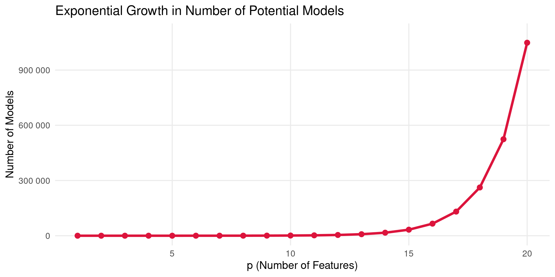
• Computational Cost: Requires fitting \(2^p\) models. This becomes computationally infeasible very quickly as \(p\) increases.

Best Subset Selection

The Catch

---

• A plot showing the number of possible subset models (\(2^p\)) versus the number of predictors (\(p\)). The number grows exponentially, rapidly exceeding millions even for modest \(p\) (e.g., \(p=20\)).

• Need more practical approaches for larger \(p\).

Ridge Regression (L2 Penalty)

---

• Idea: Shrink the OLS coefficients towards zero to reduce variance. Penalize the sum of squared coefficient values.

• Formulation: Find \(\boldsymbol{\beta}\) to minimize:

  \[ \sum_{i=1}^n (y_i - \boldsymbol{\beta}^\top \dot{\mathbf{x}}_i)^2 + \lambda ||\boldsymbol{\beta}||_2^2 \]

  where \(||\boldsymbol{\beta}||_2^2 = \sum_{j=1}^p \beta_j^2\) is the squared L2 norm¹.

• \(\lambda \ge 0\) is the tuning parameter. Controls the amount of shrinkage.

  • \(\lambda = 0 \implies\) OLS solution.
  • \(\lambda \to \infty \implies\) \(\hat{\beta}_j \to 0\) for \(j=1, \dots, p\).

1. (Intercept \(\beta_0\) is usually not penalized).

Ridge Regression

Solution

---

• Unlike Best Subset or Lasso (later), Ridge Regression has a closed-form solution:

  \[ \hat{\boldsymbol{\beta}}_{Ridge}(\lambda) = (\dot{\mathbf{X}}^\top \dot{\mathbf{X}} + \lambda \mathbf{I}^*)^{-1} \dot{\mathbf{X}}^\top \dot{\mathbf{y}} \]

  Where \(\mathbf{I}^*\) is a \((p+1) \times (p+1)\) identity matrix with the top-left element (corresponding to the intercept) set to zero to avoid penalizing \(\beta_0\).

• The term \(\lambda \mathbf{I}^*\) makes the matrix invertible even if \(\dot{\mathbf{X}}^\top \dot{\mathbf{X}}\) is singular (\(p+1 > n\)). Solves one OLS limitation.

Ridge Regression

Key Properties

---

• Reduces Variance: Especially effective when OLS coefficients are high variance (e.g., multicollinearity, high dimensions).

• Keeps All Predictors: It shrinks coefficients towards zero, but does not set them exactly to zero (unless \(\lambda = \infty\)). It does not perform variable selection.

• Requires Tuning \(\lambda\): The performance depends crucially on choosing a good value for \(\lambda\). Typically done via Cross-Validation.

• Scale Dependence: The solution depends on the scaling of predictors. It’s standard practice to standardize predictors (\(X_j\)) to have mean 0 and variance 1 before applying Ridge.

Ridge Regression in R

glmnet

---

• The glmnet package is highly efficient for fitting Ridge, Lasso.
• Requires predictors as a matrix (X) and response as a vector (y).
• alpha = 0 specifies Ridge Regression.

# --- Load Necessary Libraries ---
library(tidymodels) # Main meta-package
library(glmnet)     # The engine
library(dplyr)      # Data manipulation
library(doParallel) # Optional: For parallel processing

# --- 1. Simulate Example Data ---
set.seed(123)
n_train <- 100
p <- 20
X_train_mat <- matrix(rnorm(n_train * p), ncol = p)
true_beta <- rnorm(p) * sample(c(0, 1), p, replace = TRUE, prob = c(0.7, 0.3))
y_train_vec <- X_train_mat %*% true_beta + rnorm(n_train, sd = 1.5)
colnames(X_train_mat) <- paste0("predictor_", 1:p)
train_data <- as_tibble(X_train_mat) |> mutate(y = as.numeric(y_train_vec))

n_val <- 50
X_val_mat <- matrix(rnorm(n_val * p), ncol = p)
y_val_vec <- X_val_mat %*% true_beta + rnorm(n_val, sd = 1.5)
colnames(X_val_mat) <- paste0("predictor_", 1:p)
val_data <- as_tibble(X_val_mat) |> mutate(y = as.numeric(y_val_vec))

# --- 2. Define Model Specification ---
ridge_spec <- linear_reg(penalty = tune(), mixture = 0) |> # mixture = 0 for Ridge
  set_engine("glmnet")

# --- 3. Define Preprocessing Recipe ---
ridge_recipe <- recipe(y ~ ., data = train_data) |>
  step_normalize(all_predictors()) # Center and scale predictors

# --- 4. Create Workflow ---
ridge_workflow <- workflow() |>
  add_recipe(ridge_recipe) |>
  add_model(ridge_spec)

# --- 5. Set up Cross-Validation ---
set.seed(456)
cv_folds <- vfold_cv(train_data, v = 10)

# --- 6. Define Tuning Grid for Lambda (Penalty) ---
lambda_grid <- grid_regular(penalty(), levels = 30) # Test 30 lambda values

# --- 7. Tune the Model using Cross-Validation ---
registerDoParallel() # Use parallel processing if available
set.seed(789)
ridge_tune_results <- tune_grid(
  ridge_workflow,
  resamples = cv_folds,
  grid = lambda_grid,
  metrics = metric_set(rmse, rsq)
)
# Stop parallel backend (good practice)
stopImplicitCluster()

# --- 8. Analyze Tuning Results and Select Best Model ---

cat("\n--- Analyzing Tuning Results ---\n")
# Plot CV performance vs. lambda
tuning_plot <- autoplot(ridge_tune_results) + theme_minimal()
print(tuning_plot)

# Show the top performing hyperparameter values based on RMSE
cat("\nTop 5 Hyperparameter Sets (based on RMSE):\n")
show_best(ridge_tune_results, metric = "rmse", n = 5) |> print()

# Select the *single best* lambda based on the lowest cross-validated RMSE
best_lambda_ridge_tidy <- select_best(ridge_tune_results, metric = "rmse")
cat("\n--- Best Model Selection ---\n")
cat("The best hyperparameter value (lambda/penalty) based on minimum CV RMSE is:\n")
print(best_lambda_ridge_tidy)

# --- 9. Finalize Workflow with Best Hyperparameter ---
# Update the workflow by replacing `tune()` with the actual best lambda value found
final_ridge_workflow <- finalize_workflow(
  ridge_workflow,
  best_lambda_ridge_tidy # The parameters selected in the previous step
)
cat("\nWorkflow finalized with best lambda:\n")
print(final_ridge_workflow)

# --- 10. Fit the Final Model on the Full Training Data ---
# Now that we've chosen the best lambda using cross-validation, we train the
# model one last time on *all* the training data using that lambda.
cat("\n--- Fitting Final Model on Full Training Data ---\n")
final_ridge_fit <- fit(final_ridge_workflow, data = train_data)
cat("Final model fit object created.\n")

# --- 11. Make Predictions on New Data ---
# Use the *fitted final workflow* to make predictions on the validation set
# (or any new dataset with the same predictor columns).
# The workflow automatically applies the same preprocessing (scaling).
cat("\n--- Making Predictions on Validation Set ---\n")
predictions_ridge_tidy <- predict(final_ridge_fit, new_data = val_data)

# Combine predictions with actual validation outcomes for evaluation
val_results <- val_data |>
  select(y) |> # Actual outcome column
  bind_cols(predictions_ridge_tidy) |> # Adds the prediction column '.pred'
  rename(predicted_y = .pred, actual_y = y) # Rename for clarity

cat("Predictions generated for validation data (first 10 rows):\n")
print(head(val_results, 10))

# --- 12. Evaluate Final Model Performance on Validation Set (Optional) ---
cat("\n--- Evaluating Performance on Validation Set ---\n")
final_rmse <- rmse(val_results, truth = actual_y, estimate = predicted_y)
final_rsq <- rsq(val_results, truth = actual_y, estimate = predicted_y)

cat(sprintf("Validation RMSE: %.4f\n", final_rmse$.estimate))
cat(sprintf("Validation R-squared: %.4f\n", final_rsq$.estimate))

Lasso Regression

Least Absolute Shrinkage and Selection Operator

---

• Developed by Tibshirani (1996). Aims to improve prediction accuracy and interpretation by performing shrinkage and variable selection.

• Formulation: Find \(\boldsymbol{\beta}\) to minimize:

  \[ \sum_{i=1}^n (y_i - \boldsymbol{\beta}^\top \dot{\mathbf{x}}_i)^2 + \lambda ||\boldsymbol{\beta}||_1 \]

  where \(||\boldsymbol{\beta}||_1 = \sum_{j=1}^p |\beta_j|\) is the L1 norm¹.

1. (Intercept \(\beta_0\) is usually not penalized)

Lasso Regression

Key Properties

---

• Shrinkage: Like Ridge, Lasso shrinks coefficients towards zero.

• Variable Selection: Unlike Ridge, the L1 penalty forces some coefficients to be exactly zero for sufficiently large \(\lambda\). This performs automatic variable selection.

• Sparsity: Produces “sparse” models with fewer non-zero coefficients, which are often easier to interpret.

• Requires Tuning \(\lambda\): Performance depends on \(\lambda\), chosen via Cross-Validation.

• Scale Dependence: Standardize predictors before applying Lasso.

Why does L1 Penalty Cause Sparsity?

---

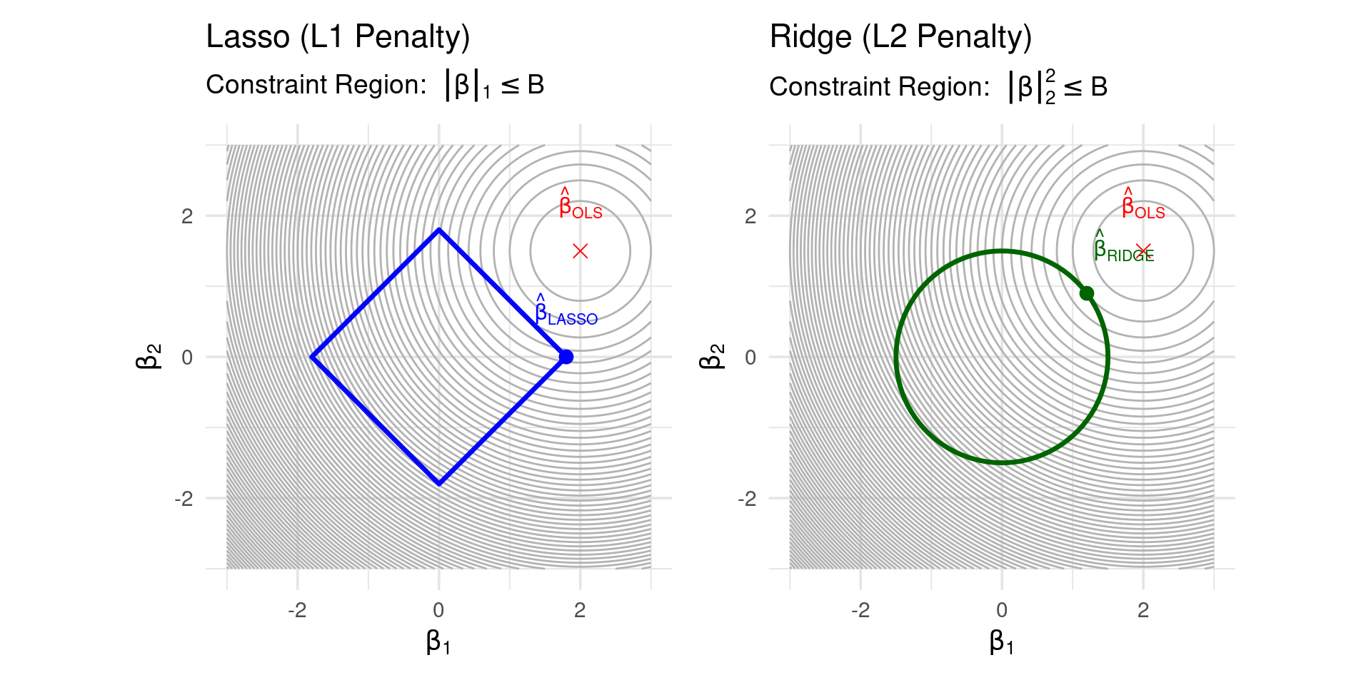
• Consider the contours of the RSS and the penalty term constraint regions:
  • Ridge (L2): Constraint \(||\boldsymbol{\beta}||_2^2 \le B\) is a circle (in 2D). RSS contours are ellipses. The solution often occurs where the ellipse touches the circle without hitting an axis.
  • Lasso (L1): Constraint \(||\boldsymbol{\beta}||_1 \le B\) is a diamond (in 2D). The corners of the diamond lie on the axes. The RSS ellipse is more likely to make its first contact with the diamond constraint region at a corner, implying one coefficient is zero.

• The L1 penalty has a “kink” at zero, while L2 is smooth.

Why does L1 Penalty Cause Sparsity?

---

Sparsity Measures Comparison

adjusted p=10

---

Coefficient Vector \(\boldsymbol{\beta}\) (p=10)	L0 Norm: \(||\boldsymbol{\beta}||_0\)	L1 Norm: \(||\boldsymbol{\beta}||_1\)	L2 Norm Sq: \(||\boldsymbol{\beta}||_2^2\)
(0, 0, 0, 0, 0, 0, 0, 0, 0, 0)	0	0.0	0.0
(0.1, 0.1, 0.1, 0.1, 0.1, 0.1, 0.1, 0.1, 0.1, 0.1)	10	1.0	0.1
(1, 1, 1, 1, 1, 1, 1, 1, 1, 1)	10	10.0	10.0
(0, 0, 0, 0, 1, 1, 0, 0, 0, 0)	2	2.0	2.0

• L0 counts non-zeros (measures sparsity directly but hard to optimize).
• L1 sums absolute values (convex proxy for sparsity).
• L2 sums squared values (penalizes large coefficients heavily, but not sparsity).

Lasso Regression in R

glmnet

---

• Use glmnet with alpha = 1.

# --- Load Necessary Libraries ---
library(tidymodels) # Main meta-package
library(glmnet)     # The engine
library(dplyr)      # Data manipulation
library(doParallel) # Optional: For parallel processing

# --- 1. Simulate Example Data ---
set.seed(123)
n_train <- 100
p <- 20
X_train_mat <- matrix(rnorm(n_train * p), ncol = p)
true_beta <- rnorm(p) * sample(c(0, 1), p, replace = TRUE, prob = c(0.7, 0.3))
y_train_vec <- X_train_mat %*% true_beta + rnorm(n_train, sd = 1.5)
colnames(X_train_mat) <- paste0("predictor_", 1:p)
train_data <- as_tibble(X_train_mat) |> mutate(y = as.numeric(y_train_vec))

n_val <- 50
X_val_mat <- matrix(rnorm(n_val * p), ncol = p)
y_val_vec <- X_val_mat %*% true_beta + rnorm(n_val, sd = 1.5)
colnames(X_val_mat) <- paste0("predictor_", 1:p)
val_data <- as_tibble(X_val_mat) |> mutate(y = as.numeric(y_val_vec))

# --- 2. Define Model Specification ---
# Change mixture to 1 for Lasso (alpha = 1 in glmnet)
lasso_spec <- linear_reg(penalty = tune(), mixture = 1) |> # mixture = 1 for Lasso
  set_engine("glmnet")

# --- 3. Define Preprocessing Recipe ---
lasso_recipe <- recipe(y ~ ., data = train_data) |>
  step_normalize(all_predictors()) # Center and scale predictors

# --- 4. Create Workflow ---
lasso_workflow <- workflow() |>
  add_recipe(lasso_recipe) |>
  add_model(lasso_spec)

# --- 5. Set up Cross-Validation ---
set.seed(456)
cv_folds <- vfold_cv(train_data, v = 10)

# --- 6. Define Tuning Grid for Lambda (Penalty) ---
lambda_grid <- grid_regular(penalty(), levels = 30) # Test 30 lambda values

# --- 7. Tune the Model using Cross-Validation ---
registerDoParallel() # Use parallel processing if available
set.seed(789)
lasso_tune_results <- tune_grid(
  lasso_workflow,
  resamples = cv_folds,
  grid = lambda_grid,
  metrics = metric_set(rmse, rsq)
)
# Stop parallel backend (good practice)
stopImplicitCluster()

# --- 8. Analyze Tuning Results and Select Best Model ---

cat("\n--- Analyzing Tuning Results ---\n")
# Plot CV performance vs. lambda
tuning_plot <- autoplot(lasso_tune_results) + theme_minimal()
print(tuning_plot)

# Show the top performing hyperparameter values based on RMSE
cat("\nTop 5 Hyperparameter Sets (based on RMSE):\n")
show_best(lasso_tune_results, metric = "rmse", n = 5) |> print()

# Select the *single best* lambda based on the lowest cross-validated RMSE
best_lambda_lasso_tidy <- select_best(lasso_tune_results, metric = "rmse")
cat("\n--- Best Model Selection ---\n")
cat("The best hyperparameter value (lambda/penalty) based on minimum CV RMSE is:\n")
print(best_lambda_lasso_tidy)

# --- 9. Finalize Workflow with Best Hyperparameter ---
# Update the workflow by replacing `tune()` with the actual best lambda value found
final_lasso_workflow <- finalize_workflow(
  lasso_workflow,
  best_lambda_lasso_tidy # The parameters selected in the previous step
)
cat("\nWorkflow finalized with best lambda:\n")
print(final_lasso_workflow)

# --- 10. Fit the Final Model on the Full Training Data ---
# Now that we've chosen the best lambda using cross-validation, we train the
# model one last time on *all* the training data using that lambda.
cat("\n--- Fitting Final Model on Full Training Data ---\n")
final_lasso_fit <- fit(final_lasso_workflow, data = train_data)
cat("Final model fit object created.\n")

# You can extract the underlying glmnet model if needed
# final_glmnet_model <- extract_fit_engine(final_lasso_fit)
# coef(final_glmnet_model) # Coefficients on the scaled scale

# --- 11. Make Predictions on New Data ---
# Use the *fitted final workflow* to make predictions on the validation set
# (or any new dataset with the same predictor columns).
# The workflow automatically applies the same preprocessing (scaling).
cat("\n--- Making Predictions on Validation Set ---\n")
predictions_lasso_tidy <- predict(final_lasso_fit, new_data = val_data)

# Combine predictions with actual validation outcomes for evaluation
val_results <- val_data |>
  select(y) |> # Actual outcome column
  bind_cols(predictions_lasso_tidy) |> # Adds the prediction column '.pred'
  rename(predicted_y = .pred, actual_y = y) # Rename for clarity

cat("Predictions generated for validation data (first 10 rows):\n")
print(head(val_results, 10))

# --- 12. Evaluate Final Model Performance on Validation Set (Optional) ---
cat("\n--- Evaluating Performance on Validation Set ---\n")
final_rmse <- rmse(val_results, truth = actual_y, estimate = predicted_y)
final_rsq <- rsq(val_results, truth = actual_y, estimate = predicted_y)

cat(sprintf("Validation RMSE: %.4f\n", final_rmse$.estimate))
cat(sprintf("Validation R-squared: %.4f\n", final_rsq$.estimate))

Ridge vs. Lasso Summary

---

Feature	Ridge Regression (L2)	Lasso (L1)
Penalty	\(\lambda \sum \beta_j^2\)	\(\lambda \sum |\beta_j|\)
Shrinkage	Yes	Yes
Variable Select	No (keeps all predictors)	Yes (sets some coefficients to zero)
Sparsity	No	Yes
Solution	Closed-form	No closed-form (iterative algorithms)
Computation	Very Fast	Fast (convex optimization)
Use Case	Prediction, multicollinearity	Prediction, Interpretation, Feature Select.
High \(p\) (\(p>n\))	Works well	Can struggle if \(p>>n\) (selects \(\le n\))

Choosing the Right Method

---

• Prediction Accuracy: Often Lasso, Ridge perform best, tuned via CV. Best Subset can be good if \(p\) is small enough.

• Model Interpretability / Feature Selection: Lasso is preferred due to sparsity. Best Subset/Stepwise also select variables but can be less stable. Ridge is not suitable as it keeps all variables.

• Computational Cost: Ridge and Lasso are generally much faster than Best Subset or Stepwise, especially for large \(p\).

• Case \(p > n\): Ridge works well. Lasso selects at most \(n\) variables. Best Subset/Stepwise are generally applicable but computationally costly.

Conclusion

---

• Linear models can be extended to high-dimensional settings (\(p > n\) or large \(p\)) using regularization techniques (Ridge, Lasso).

• These methods manage the bias-variance trade-off, improving predictive performance over OLS.

• Lasso provides the additional benefit of automatic variable selection, leading to sparse and interpretable models.

• Choosing the tuning parameter (\(\lambda\)) via Cross-Validation is essential.

• Understanding these methods provides a foundation for tackling complex, high-dimensional data problems.

References

---

Basics

• Aprendizado de Máquina: uma abordagem estatística, Izbicki, R. and Santos, T. M., 2020, link: https://rafaelizbicki.com/AME.pdf.

• An Introduction to Statistical Learning: with Applications in R, James, G., Witten, D., Hastie, T. and Tibshirani, R., Springer, 2013, link: https://www.statlearning.com/.

• Mathematics for Machine Learning, Deisenroth, M. P., Faisal. A. F., Ong, C. S., Cambridge University Press, 2020, link: https://mml-book.com.

References

---

Complementaries

• An Introduction to Statistical Learning: with Applications in python, James, G., Witten, D., Hastie, T. and Tibshirani, R., Taylor, J., Springer, 2023, link: https://www.statlearning.com/.

• Matrix Calculus (for Machine Learning and Beyond), Paige Bright, Alan Edelman, Steven G. Johnson, 2025, link: https://arxiv.org/abs/2501.14787.

• Machine Learning Beyond Point Predictions: Uncertainty Quantification, Izibicki, R., 2025, link: https://rafaelizbicki.com/UQ4ML.pdf.

• Mathematics of Machine Learning, Petersen, P. C., 2022, link: http://www.pc-petersen.eu/ML_Lecture.pdf.