Statistical Machine Learning
Continuos Optimization
UFPE
Motivation: Optimization in Statistical Machine Learning
- Statistical Machine Learning models learn by finding optimal parameters (weights, biases, etc.).
- “Optimal” means parameters that minimize (or maximize) an objective function (e.g., loss function, likelihood).
- Training = Optimization Problem: Find the parameter values \(\boldsymbol{\theta}\) that minimize a loss \(L(\boldsymbol{\theta})\).
Goal: Given an objective function, find the best set of parameters.
Continuous vs. Discrete Optimization
- Continuous Optimization: Parameters live in a continuous space (e.g., \(\mathbb{R}^p\)). This is the focus today.
- Examples: Linear Regression parameters.
- We often deal with differentiable objective functions.
- Discrete/Combinatorial Optimization: Parameters or decisions come from a discrete set.
- Examples: Feature selection, finding the best path (graph problems).
- Uses different techniques (e.g., search algorithms, integer programming).
Focus: Continuous, differentiable objective functions.
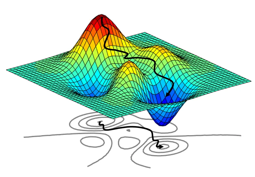
The Landscape: Objective Functions
Imagine the objective function \(f(\boldsymbol{\theta})\) as a landscape over the parameter space \(\boldsymbol{\Theta}\).
- Goal: Find the lowest point (minimum value).
- Gradients (\(\nabla f\)): Point uphill in the direction of steepest ascent.
- Intuition: To find a valley, move in the opposite direction of the gradient (downhill).
Example: A 1D Function
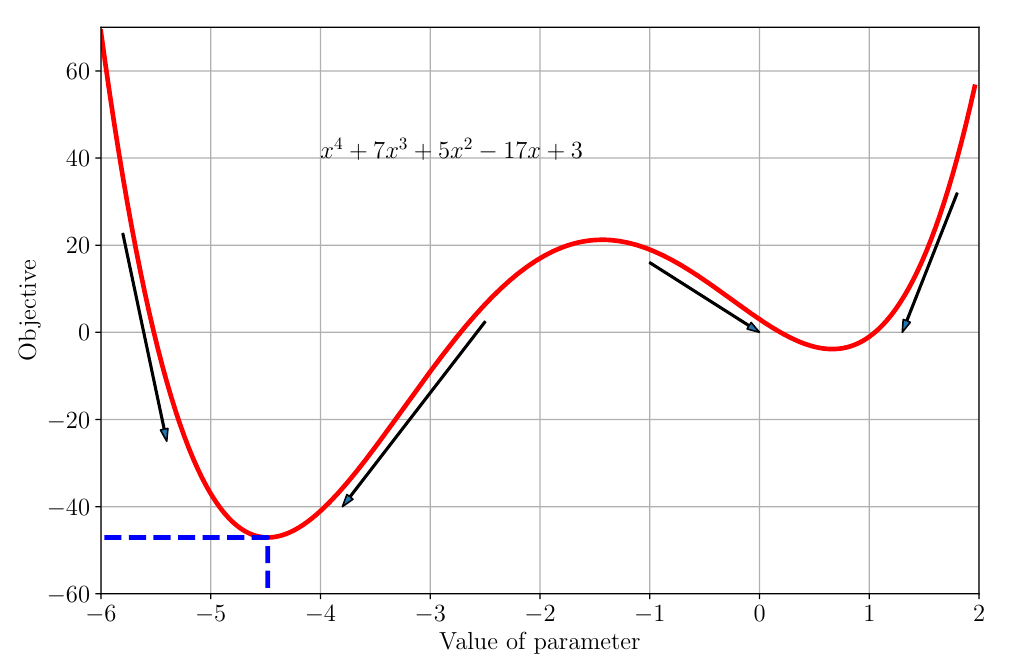
- Function: \(f(\theta) = \theta^4 + 7\theta^3 + 5\theta^2 - 17\theta + 3\)
- Global Minimum: Lowest point overall (around \(\theta \approx -4.5\)).
- Local Minimum: Lowest point in its neighborhood (around \(\theta \approx 0.7\)).
- Gradients: Arrows indicate the negative gradient (downhill direction).
Finding Minima Analytically
- Stationary Points: Points where the gradient (derivative in 1D) is zero.
- \(\frac{dl(\theta)}{d\theta} = 4\theta^3 + 21\theta^2 + 10\theta - 17\)
- Setting \(\frac{dl(\theta)}{d\theta} = 0\) gives potential minima, maxima, or saddle points.
- Second Derivative Test:
- \(\frac{d^2l(\theta)}{d\theta^2} = 12\theta^2 + 42\theta + 10\)
- If \(\frac{d^2l}{d\theta^2} > 0\) at a stationary point \(\implies\) Local Minimum.
- If \(\frac{d^2l}{d\theta^2} < 0\) at a stationary point \(\implies\) Local Maximum.
- If \(\frac{d^2l}{d\theta^2} = 0 \implies\) Inconclusive.
Finding Minima Analytically

Challenge: Analytically solving \(\nabla f(\boldsymbol{\theta}) = \mathbf{0}\) is often impossible for complex ML model.
Finding Minima Analytically
.png)
Numerical Optimization:
The Need for Iteration
Since we usually can’t solve for the minimum directly, we use iterative methods.
- Start at an initial guess \(\boldsymbol{\theta}_0\).
- Repeatedly update the guess to move towards lower function values.
Key Idea: Use the gradient to guide the updates.
Continuous Optimization
- Gradient Descent;
- Gradient Descent with Momentum;
- Stochastic Gradient Descent;
- Constrained Optimization;
- Lagrange Multipliers;
Optimization Using Gradient Descent
We want to find the minimum of a function \(f(\boldsymbol{\theta})\) where \(\boldsymbol{\theta} \in \mathbb{R}^p\), i.e., find \[\min_{\boldsymbol{\theta} \in \mathbb{R}^p} f(\boldsymbol{\theta})\] where \(f\) is differentiable.
Gradient descent is a first-order optimization algorithm.
To find a local minimum of a function using gradient descent, one takes steps proportional to the negative of the gradient of the function at the current point.
- The gradient \(\nabla f(\boldsymbol{\theta})\) points in the direction of steepest ascent.
- The negative gradient \(-\nabla f(\boldsymbol{\theta})\) points in the direction of steepest descent.
Optimization Using Gradient Descent
Algorithm:
- Start at \(\boldsymbol{\theta}_0\).
- but, in general case, iterate: \[ \boldsymbol{\theta}_{i+1} = \boldsymbol{\theta}_i - \gamma_i (\nabla f(\boldsymbol{\theta}_i))^\top \]
- \(\boldsymbol{\theta}_i\): Current parameter estimate.
- \(\nabla f(\boldsymbol{\theta}_i)\): Gradient of \(f\) at \(\boldsymbol{\theta}_i\).
- \(\gamma_i\): Step size (or learning rate) at iteration \(i\). Usually \(\gamma_i = \gamma > 0\).
If \(\gamma\) is small enough and \(\gamma_i (\nabla f(\boldsymbol{\theta}_i))^\top \geq 0\), \(f(\boldsymbol{\theta}_{i+1}) \le f(\boldsymbol{\theta}_i)\).
Optimization Using Gradient Descent
Example:
\[f(\theta) = \theta (\theta - 1)\]
What is the value of \(\theta\) that minimizes this function?
Optimization Using Gradient Descent
Example 2:
Seja \(\theta = (x,y)\), e
\[f(x,y) = (x-2)^2 + (y + 1)^2\]
Optimization Using Gradient Descent
Example: 2D Quadratic Function
Minimize \(f(\theta_1, \theta_2) = \frac{1}{2} \begin{bmatrix} \theta_1 \\ \theta_2 \end{bmatrix}^\top \begin{bmatrix} 2 & 1 \\ 1 & 20 \end{bmatrix} \begin{bmatrix} \theta_1 \\ \theta_2 \end{bmatrix} - \begin{bmatrix} 5 \\ 3 \end{bmatrix}^\top \begin{bmatrix} \theta_1 \\ \theta_2 \end{bmatrix}\)
Gradient: \(\nabla f(\theta_1, \theta_2) = \begin{bmatrix} \theta_1 \\ \theta_2 \end{bmatrix}^\top \begin{bmatrix} 2 & 1 \\ 1 & 20 \end{bmatrix} - \begin{bmatrix} 5 \\ 3 \end{bmatrix}^\top\)
Update Rule (using \(\boldsymbol{\theta} = [\theta_1, \theta_2]^\top\)): \[ \boldsymbol{\theta}_{i+1} = \boldsymbol{\theta}_i - \gamma \left( \begin{bmatrix} 2 & 1 \\ 1 & 20 \end{bmatrix} \boldsymbol{\theta}_i - \begin{bmatrix} 5 \\ 3 \end{bmatrix} \right) \]
(Note: We use column vector form here for calculation)
Optimization Using Gradient Descent
Example: 2D Quadratic Function
- Start at \(\boldsymbol{\theta}_0 = [-3, -1]^\top\). Step size \(\gamma = 0.085\).
- What is the of \(\boldsymbol{\theta}_1\) value?
\[ \boldsymbol{\theta}_{1} = \begin{bmatrix} -3 \\ -1 \end{bmatrix} - 0.085 \left( \begin{bmatrix} 2 & 1 \\ 1 & 20 \end{bmatrix} \begin{bmatrix} -3 \\ -1 \end{bmatrix} - \begin{bmatrix} 5 \\ 3 \end{bmatrix} \right) \]
\[ \boldsymbol{\theta}_{1} = \begin{bmatrix} -3 \\ -1 \end{bmatrix} - 0.085 \left( \begin{bmatrix} -7 \\ -23 \end{bmatrix} - \begin{bmatrix} 5 \\ 3 \end{bmatrix} \right) \]
\[ \boldsymbol{\theta}_{1} = \begin{bmatrix} -3 \\ -1 \end{bmatrix} - 0.085 \left( \begin{bmatrix} -12 \\ -26 \end{bmatrix} \right) \]
Optimization Using Gradient Descent
Example: 2D Quadratic Function
\[ \boldsymbol{\theta}_{1} = \begin{bmatrix} -3 \\ -1 \end{bmatrix} - \begin{bmatrix} - 1.02 \\ -2.21 \end{bmatrix} \]
\[ \boldsymbol{\theta}_{1} = \begin{bmatrix} -1.98 \\ 1.21 \end{bmatrix} \]
Optimization Using Gradient Descent
Example: 2D Quadratic Function
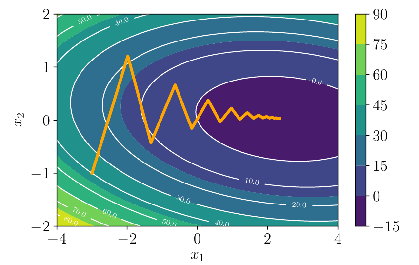
Gradient Descent on Quadratic Surface
Optimization Using Gradient Descent
Example: 2D Quadratic Function
The Step Size (\(\gamma\))
Also called the learning rate.
Too Small \(\gamma\): Very slow convergence. Many steps needed.
Too Large \(\gamma\): Overshooting the minimum, oscillations, divergence (function value increases).
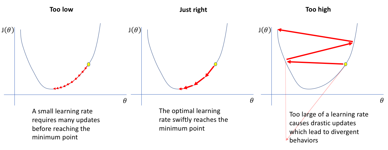
Effect of learning rate - https://www.jeremyjordan.me
The Step Size (\(\gamma\))
Choosing the Step Size
- Fixed \(\gamma\): Simplest approach, requires tuning.
- Decreasing \(\gamma\): Start larger, decrease over time (e.g., \(\gamma_i = \gamma_0 / (1+ki)\)). Common in deep learning.
- Adaptive Methods: Adjust \(\gamma\) based on the optimization progress.
- Heuristic:
- If \(f(\boldsymbol{\theta}_{i+1}) > f(\boldsymbol{\theta}_i)\) (value increased): Undo step, decrease \(\gamma\).
- If \(f(\boldsymbol{\theta}_{i+1}) < f(\boldsymbol{\theta}_i)\) (value decreased): Maybe increase \(\gamma\).
- More sophisticated methods exist (AdaGrad, RMSProp, Adam - beyond this chapter).
- Heuristic:
- Line Search: Find the optimal \(\gamma_i\) at each step that minimizes \(f(\boldsymbol{\theta}_i - \gamma \nabla f(\boldsymbol{\theta}_i))\) along the gradient direction. Can be expensive.
Gradient Descent with Momentum
Gradient Descent with Momentum
- Idea: Introduce a “velocity” term \(\Delta \boldsymbol{\theta}_i\) that accumulates past gradients. Update depends on current gradient and previous direction.
- Update Rules: \[
\Delta \boldsymbol{\theta}_{i+1} = \alpha \Delta \boldsymbol{\theta}_i - \gamma (\nabla f(\boldsymbol{\theta}_i))^\top \quad (\text{Velocity update})
\] \[
\boldsymbol{\theta}_{i+1} = \boldsymbol{\theta}_i + \Delta \boldsymbol{\theta}_{i+1} \quad (\text{Position update})
\]
- \(\alpha \in [0,1]\): Momentum parameter (e.g., 0.9), decay factor for past velocity.
- \(\Delta \boldsymbol{\theta}_i\): Change in \(\boldsymbol{\theta}\) from step \(i-1\) to \(i\), i.e., \[\Delta \boldsymbol{\theta}_i = \boldsymbol{\theta}_i - \boldsymbol{\theta}_{i-1} = \alpha \Delta \boldsymbol{\theta}_{i-1} - \gamma (\nabla f(\boldsymbol{\theta}_{i-1}))^\top\]
A higher α gives more importance to the past, preserving more of the previous velocity in updates.
Momentum: Intuition
- Like a heavy ball rolling down the hill.
- Builds up speed in consistent downhill directions.
- Averages out oscillating gradient components.
- Helps pass through small local minima or flat regions.
Momentum vs GD - https://cs231n.github.io/neural-networks-3/
Computational Cost
- Objective function in ML often a sum over n data points: \[
\mathcal{L}(\boldsymbol{\theta}) = \frac{1}{n} \sum_{i=1}^n \mathcal{L}_i(\boldsymbol{\theta})\]
- \(\mathcal{L}_i(\boldsymbol{\theta})\): Loss for the \(i\)-th data point \((\boldsymbol{\theta}_i, y_i)\).
- Gradient is also a sum: \[ \nabla \mathcal{L}(\boldsymbol{\theta}) = \frac{1}{n} \sum_{i=1}^n \nabla \mathcal{L}_i(\boldsymbol{\theta}) \]
- Calculating the full gradient requires iterating through the entire dataset at each step.
- Impractical for large datasets (e.g., millions of images).
Stochastic Gradient Descent (SGD)
Stochastic Gradient Descent (SGD)
- Idea: Approximate the full gradient using just one or a small batch of data points at each step.
- Single Point SGD:
- Pick a random data point \(i\) from \(\{1, \ldots, n\}\).
- Update using only the gradient for that point: \[ \boldsymbol{\theta}_{i+1} = \boldsymbol{\theta}_i - \gamma_i (\nabla \mathcal{L}_i(\boldsymbol{\theta}_i))^\top \]
- Mini-batch SGD (Most Common):
- Pick a random mini-batch \(\mathcal{B}\) of size \(B\) (e.g., \(B=32, 64, \ldots\)) from \(\{1, \ldots, n\}\).
- Update using the average gradient over the mini-batch: \[ \boldsymbol{\theta}_{i+1} = \boldsymbol{\theta}_i - \gamma_i \left( \frac{1}{B} \sum_{i \in \mathcal{B}} \nabla \mathcal{L}_i(\boldsymbol{\theta}_i) \right)^\top \]
SGD: Why Does it Work?
- On average, the stochastic gradient points in the same direction as the true gradient.
- Much faster updates: Cost per step is proportional to \(B\), not \(n\).
- Noisy Gradients: The path taken is much noisier than full batch GD.
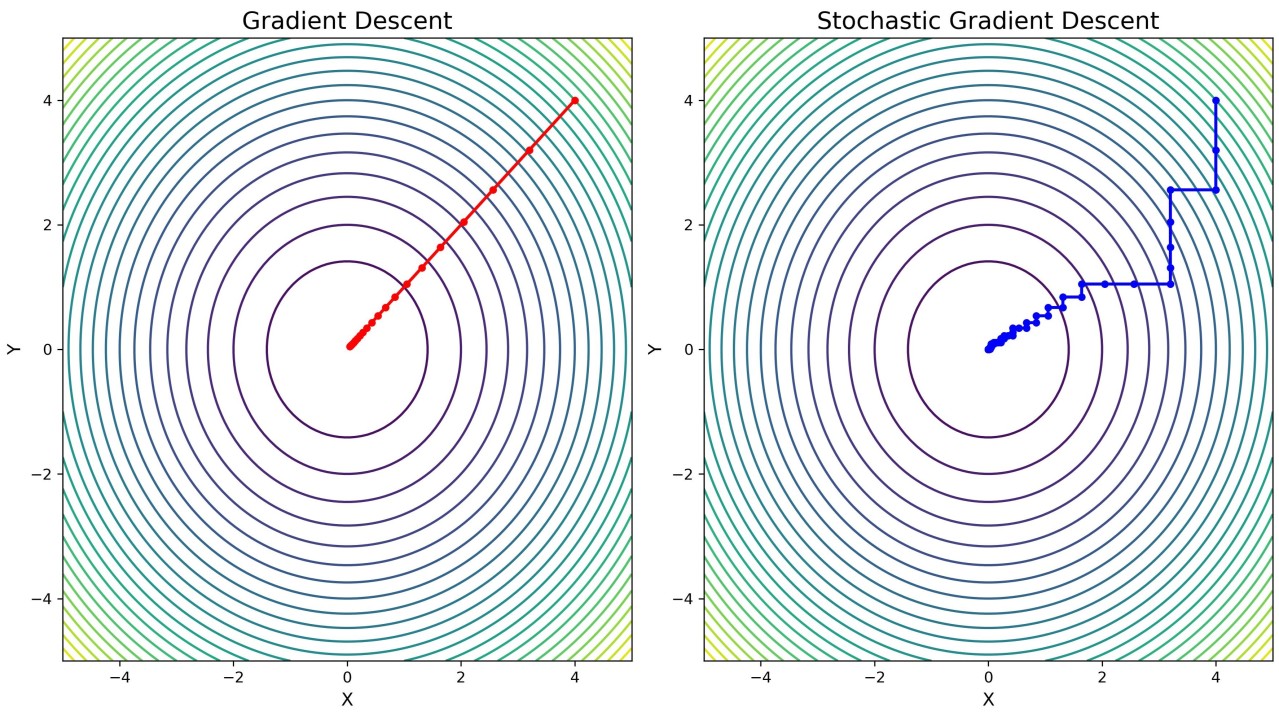
SGD vs GD Path - pulse/gradient-descent-gd-stochastic-sgd-vekil-bekmyradov-qvs4e/
SGD: Pros and Cons
Pros:
- Computationally efficient: Scales to massive datasets.
- Faster initial progress: Can make updates more frequently.
- Noise can help escape local minima: The randomness might bump the parameters out of shallow local optima.
- Often leads to better generalization (performance on unseen data), perhaps because it finds “flatter” minima.
Cons:
- Noisy updates: Convergence can be erratic, may not settle precisely at the minimum. Requires careful tuning of learning rate schedule (decreasing \(\gamma\)).
- Higher variance in parameter updates compared to batch GD. Mini-batch size \(B\) controls this trade-off.
Constrained Optimization
Constrained Optimization
Find \(\min_{\boldsymbol{\theta}} f(\boldsymbol{\theta})\) subject to constraints, where \(f: \mathbb{R}^p \rightarrow \mathbb{R}\).
- Often, parameters \(\boldsymbol{\theta}\) or functions of them must satisfy certain conditions.
- Standard Form: \[
\min_{\boldsymbol{\theta}} f(\boldsymbol{\theta})
\] \[
\text{subject to } \quad g_i(\boldsymbol{\theta}) \le 0 \quad \text{for } i = 1, \ldots, m
\] \[
\quad \quad \quad \quad h_j(\boldsymbol{\theta}) = 0 \quad \text{for } j = 1, \ldots, p
\]
- \(f\): Objective function.
- \(g_i\): Inequality constraint functions.
- \(h_j\): Equality constraint functions.
Visualizing Constraints
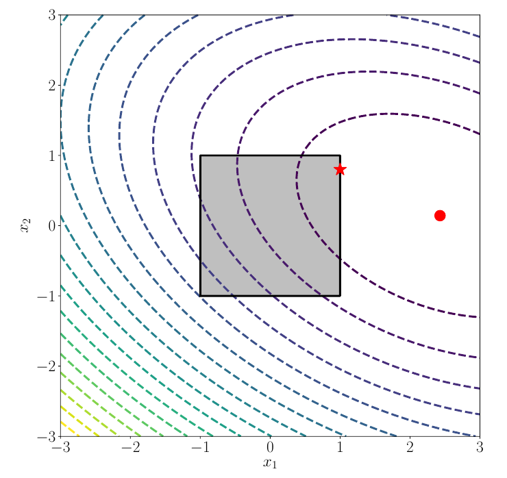
Constrained Optimization Illustration
- Feasible Region (gray region): The set of points \(\boldsymbol{\theta}\) satisfying all constraints.
- The unconstrained minimum (red circle) might be outside the feasible region.
- The constrained minimum (red star) occurs within or on the boundary of the feasible region.
Constrained Optimization
Convert to unconstrained by adding infinite penalties: \[ \min_{\boldsymbol{\theta}} J(\boldsymbol{\theta}) = f(\boldsymbol{\theta}) + \sum_{i=1}^m \mathbf{1}(g_i(\boldsymbol{\theta})) + \sum_{j=1}^p \mathbf{1}_{=0}(h_j(\boldsymbol{\theta})) \] where \(\mathbf{1}(z) = \begin{cases} 0 & \text{if } z \le 0 \\ \infty & \text{if } z > 0 \end{cases}\) and \(\mathbf{1}_{=0}(z) = \begin{cases} 0 & \text{if } z = 0 \\ \infty & \text{if } z \ne 0 \end{cases}\),
\(g_i: \mathbb{R}^p \rightarrow \mathbb{R}\) and \(h_j: \mathbb{R}^p \rightarrow \mathbb{R}\)
Problem: This new objective \(J(\boldsymbol{\theta})\) is non-differentiable and hard to optimize directly.
The Challenge:
Constrained Optimization
Our Goal
We often want to minimize (or maximize) a function \(f(\boldsymbol{\theta})\)…
…but \(\boldsymbol{\theta}\) isn’t free! It must satisfy certain constraints:
- Equality Constraints: \(h_j(\boldsymbol{\theta}) = 0\)
- Inequality Constraints: \(g_i(\boldsymbol{\theta}) \le 0\)
Why is this hard?
- Directly applying methods like Gradient Descent doesn’t easily handle the boundaries defined by constraints.
- We need a way to incorporate the constraints into the optimization process.
The Core Idea:
Lagrange Multipliers
Analogy: Penalties
- Imagine the constraints \(g_i(\boldsymbol{\theta}) \le 0\) define a “feasible region” where solutions are allowed.
- We want to stay inside or on the boundary of this region.
- Idea: Instead of treating constraints as rigid walls (“hard constraints”), let’s add a penalty to our objective function \(f(\boldsymbol{\theta})\) if we violate a constraint (“soft constraint”).
Lagrange Multipliers (λ)
- Introduce a non-negative variable \(\lambda_i \ge 0\) for each inequality constraint \(g_i(\boldsymbol{\theta}) \le 0\).
- This \(\lambda_i\) acts like the price or penalty rate for violating the \(i\)-th constraint.
Constructing The Lagrangian
Inequality Constraints
For the problem: \(\min f(\boldsymbol{\theta})\) subject to \(g_i(\boldsymbol{\theta}) \le 0\) for \(i=1, \ldots, m\)
We combine the objective and the weighted constraints into a single function:
The Lagrangian Function:
\[ \mathcal{L}(\boldsymbol{\theta}, \boldsymbol{\lambda}) = f(\boldsymbol{\theta}) + \sum_{i=1}^m \lambda_i g_i(\boldsymbol{\theta}) \]
- \(\boldsymbol{\theta}\): The original primal variables we want to find.
- \(\boldsymbol{\lambda} = [\lambda_1, \ldots, \lambda_m]^T\): The Lagrange multipliers (or dual variables). One \(\lambda_i\) for each \(g_i\).
- Crucial Requirement: We enforce \(\lambda_i \ge 0\) for all \(i\).
Why \(\lambda_i \ge 0\)?
The Penalty Intuition
Consider one term in the Lagrangian sum: \(\lambda_i g_i(\boldsymbol{\theta})\), where \(\lambda_i \ge 0\).
Goal: Minimize \(\mathcal{L}(\boldsymbol{\theta}, \boldsymbol{\lambda})\) with respect to \(\boldsymbol{\theta}\)
- Case 1: Constraint Satisfied (\(g_i(\boldsymbol{\theta}) < 0\))
- We are safely inside the feasible region for this constraint.
- The term \(g_i(\boldsymbol{\theta})\) is negative.
- To minimize \(\mathcal{L}\), the optimization will push \(\lambda_i\) towards zero. Why pay a penalty if you don’t need to? \(\implies \lambda_i g_i(\boldsymbol{\theta}) = 0\).
- Case 2: Constraint Active (\(g_i(\boldsymbol{\theta}) = 0\))
- We are exactly on the boundary.
- The term \(g_i(\boldsymbol{\theta})\) is zero, so \(\lambda_i g_i(\boldsymbol{\theta}) = 0\).
- \(\lambda_i\) can be positive, representing the “cost” or sensitivity of \(f(\boldsymbol{\theta})\) to this constraint.
Why \(\lambda_i \ge 0\)?
The Penalty Intuition
- Case 3: Constraint Violated (\(g_i(\boldsymbol{\theta}) > 0\))
- We are outside the feasible region.
- The term \(g_i(\boldsymbol{\theta})\) is positive.
- Since \(\lambda_i \ge 0\), the term \(\lambda_i g_i(\boldsymbol{\theta})\) adds a positive penalty to \(\mathcal{L}\).
- Minimizing \(\mathcal{L}\) will push \(\boldsymbol{\theta}\) back towards the feasible region to reduce this penalty. The larger \(\lambda_i\) is, the stronger the push.
Key Point: \(\lambda_i \ge 0\) ensures we penalize violations (\(g_i > 0\)) and don’t reward them.
The Lagrangian
in Vector Form & Connection
Vector Notation
We can write the Lagrangian more compactly using vectors:
Let \(\mathbf{g}(\boldsymbol{\theta}) = [g_1(\boldsymbol{\theta}), ..., g_m(\boldsymbol{\theta})]^T\) be the vector of constraint functions.
\[ \mathcal{L}(\boldsymbol{\theta}, \boldsymbol{\lambda}) = f(\boldsymbol{\theta}) + \boldsymbol{\lambda}^T \mathbf{g}(\boldsymbol{\theta}) \quad (\text{where } \boldsymbol{\lambda} \ge \mathbf{0}) \]
- \(\boldsymbol{\lambda}^T \mathbf{g}(\boldsymbol{\theta})\) is the dot product: \(\lambda_1 g_1(\boldsymbol{\theta}) + ... + \lambda_m g_m(\boldsymbol{\theta})\).
Primal and Dual Problems
- Primal Problem (Original): \[ p^* = \min_{\boldsymbol{\theta}} \max_{\boldsymbol{\lambda} \ge 0} \mathcal{L}(\boldsymbol{\theta}, \boldsymbol{\lambda}) \] (Note: \(\max_{\boldsymbol{\lambda} \ge 0} \mathcal{L}(\boldsymbol{\theta}, \boldsymbol{\lambda})\) equals \(f(\boldsymbol{\theta})\) if constraints met, \(\infty\) otherwise.).
- Lagrange Dual Function: \[ \mathcal{D}(\boldsymbol{\lambda}) = \min_{\boldsymbol{\theta}} \mathcal{L}(\boldsymbol{\theta}, \boldsymbol{\lambda}) \]
- Dual Problem: \[ d^* = \max_{\boldsymbol{\lambda} \ge 0} \mathcal{D}(\boldsymbol{\lambda}) = \max_{\boldsymbol{\lambda} \ge 0} \min_{\boldsymbol{\theta}} \mathcal{L}(\boldsymbol{\theta}, \boldsymbol{\lambda}) \]
Weak Duality
- For any optimization problem formulated this way: \[ d^* = \max_{\boldsymbol{\lambda} \ge 0} \min_{\boldsymbol{\theta}} \mathcal{L}(\boldsymbol{\theta}, \boldsymbol{\lambda}) \le \min_{\boldsymbol{\theta}} \max_{\boldsymbol{\lambda} \ge 0} \mathcal{L}(\boldsymbol{\theta}, \boldsymbol{\lambda}) = p^* \] The optimal value of the dual problem is always less than or equal to the optimal value of the primal problem.
Why Convexity?
If the optimization problem is convex:
- Local minima are global minima: Any minimum found is the best possible solution. GD/SGD won’t get stuck in suboptimal local minima.
- Strong duality often holds: Primal optimal value equals dual optimal value (\(p^*=d^*\)), under mild conditions (like Slater’s condition). Allows solving the (potentially easier) dual problem.
- Efficient algorithms exist with theoretical guarantees.
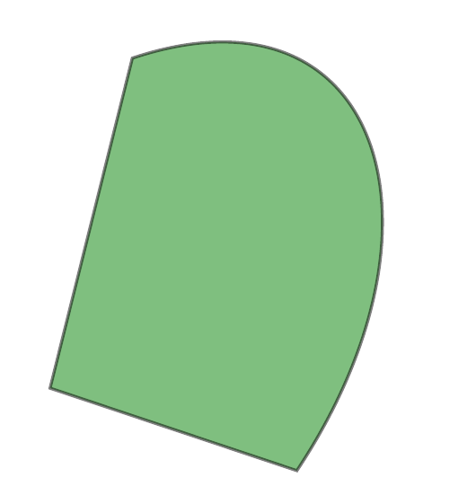
Convex Sets
A set \(C\) is convex if for any \(\boldsymbol{\theta}, \mathbf{y} \in C\) and any \(t \in [0, 1]\), the line segment connecting them is also in \(C\): \[ t \boldsymbol{\theta} + (1-t) \mathbf{y} \in C \]

Convex Functions
A function \(f: \mathbb{R}^p \to \mathbb{R}\) is convex if its domain is a convex set and for any \(\boldsymbol{\theta}, \mathbf{y}\) in its domain and \(t \in [0, 1]\): \[ f(t \boldsymbol{\theta} + (1-t) \mathbf{y}) \le t f(\boldsymbol{\theta}) + (1-t) f(\mathbf{y}) \] The function value on the line segment lies below the line segment connecting the function values at the endpoints. (The chord lies above the function).

- A function \(f\) is concave if \(-f\) is convex.
Convex Functions
Let the function \(f(x) = x^2\), assume the values \(\theta = 2\), \(y = 3\), and \(t = 0.5\), and verify whether the function \(f(x)\) is convex:
\[ f(t \theta + (1-t) y) \le t f(\theta) + (1-t) f(y) \]
Properties of Convex Functions
- First-order condition (if differentiable): \[ f(\mathbf{y}) \ge f(\boldsymbol{\theta}) + (\nabla f(\boldsymbol{\theta}))^T (\mathbf{y} - \boldsymbol{\theta}) \]
Second-order condition (if twice differentiable): \[ \nabla^2 f(\boldsymbol{\theta}) \succeq 0 \quad (\text{Hessian matrix is positive semidefinite}) \] Curvature is non-negative in all directions.
A positive semidefinite Hermitian matrix is a Hermitian matrix for which the Hermitian form \(\boldsymbol{\theta}^*A\boldsymbol{\theta}\) yields a real number greater than or equal to zero for any vector \(\boldsymbol{\theta}\).
\(\boldsymbol{\theta}^*\) represents the conjugate transpose of the vector \(\boldsymbol{\theta}\), which is obtained by transposing the vector and taking the complex conjugate of each of its elements.
Properties of Convex Functions
- Second-order condition (if twice differentiable): \[ \nabla^2 f(\boldsymbol{\theta}) \succeq 0 \quad (\text{Hessian matrix is positive semidefinite}) \] Curvature is non-negative in all directions.
A positive semidefinite Hermitian matrix is a Hermitian matrix for which the Hermitian form \(\boldsymbol{\theta}^*A\boldsymbol{\theta}\) yields a real number greater than or equal to zero for any vector \(\boldsymbol{\theta}\).
\(\boldsymbol{\theta}^*\) represents the conjugate transpose of the vector \(\boldsymbol{\theta}\), which is obtained by transposing the vector and taking the complex conjugate of each of its elements.
Example:
Negative Entropy
\[f(x) = x \log x \text{ for } x > 0\]
Consider \(y = 4\) and \(\theta = 5\),
\[ f(y) \ge f(\theta) + (\nabla f(\theta))^T (y - \theta) \]
- \(f(4) = 4 \log 4 \approx 5.55\)
\(\nabla f(\theta) = \log \theta + 1\)
\(f(\theta) + (\nabla f(\theta)) (y - \theta)\) = ???
Conclusion
- Continuous optimization provides the engine for training many Statistical Machine Learning models.
- Gradient Descent and its stochastic variants are the workhorses, especially for large-scale problems.
- Understanding constraints, duality, and convexity is crucial for formulating problems correctly and leveraging powerful theoretical guarantees when applicable.
References
Basics
Aprendizado de Máquina: uma abordagem estatística, Izibicki, R. and Santos, T. M., 2020, link: https://rafaelizbicki.com/AME.pdf.
An Introduction to Statistical Learning: with Applications in R, James, G., Witten, D., Hastie, T. and Tibshirani, R., Springer, 2013, link: https://www.statlearning.com/.
Mathematics for Statistical Machine Learning, Deisenroth, M. P., Faisal. A. F., Ong, C. S., Cambridge University Press, 2020, link: https://mml-book.com.
References
Complementaries
An Introduction to Statistical Learning: with Applications in python, James, G., Witten, D., Hastie, T. and Tibshirani, R., Taylor, J., Springer, 2023, link: https://www.statlearning.com/.
Matrix Calculus (for Statistical Machine Learning and Beyond), Paige Bright, Alan Edelman, Steven G. Johnson, 2025, link: https://arxiv.org/abs/2501.14787.
Statistical Machine Learning Beyond Point Predictions: Uncertainty Quantification, Izibicki, R., 2025, link: https://rafaelizbicki.com/UQ4ML.pdf.
Mathematics of Statistical Machine Learning, Petersen, P. C., 2022, link: http://www.pc-petersen.eu/ML_Lecture.pdf.
Statistical Machine Learning - Prof. Jodavid Ferreira