In Statistical Machine Learning, we build models to make predictions on new, unseen data.
How do we know how well our model will perform on this unseen data?
We need ways to estimate the test error1: the average error when applying our model to new observations.
Simply using the training error (error on the data used to build the model) is often misleadingly optimistic. Models can overfit the training data.
Introduction to Resampling Methods
What are they? Tools involving repeatedly drawing samples from a training dataset (\(\dot{\mathbf{X}}, \mathbf{y}\)) and refitting a model of interest on each sample.
Why use them? To obtain additional information about the fitted model that wouldn’t be available from fitting it only once on the original training data.
Examples:
Estimate the variability of a linear regression fit.
Estimate the test error of a model.
Select the appropriate level of model flexibility.
Introduction to Resampling Methods
Trade-off: Can be computationally expensive (fitting the same method multiple times), but modern computing power often makes this feasible.
Focus: We’ll cover the one most common method:
Cross-Validation
Model Assessment vs. Model Selection
Model Assessment:
Evaluating a final chosen model’s performance.
Goal: Estimate its test error rate on new data.
Example:
We decided on a quadratic model;
How well will it predict mpg for new cars?
Model Assessment vs. Model Selection
Model Selection:
Selecting the proper level of flexibility for a model.
Goal: Choose the best model among a set of candidates by estimating their test errors and picking the one with the lowest estimated test error.
Example:
Should we use a linear, quadratic, or cubic model for mpg prediction?
Which one is likely to have the lowest error on new data?
Resampling methods are crucial for both tasks.
The Challenge: Estimating Test Error
Recall Training Error: The average loss over the training sample \((\dot{\mathbf{X}}, \dot{\mathbf{y}})\).
Recall Test Error: The average error from using our method to predict the response \(Y\) on a new observation \((\dot{\mathbf{x}}_0, y_0)\) not used in training.
Regression (Quantitative \(Y\)): Typically \((y_0 - \hat{f}(\mathbf{x}_0))^2\) (Test SE)
Classification (Qualitative \(Y\)): Typically \(I(y_0 \neq \hat{y}_0)\) (Test Error)
The Challenge: Estimating Test Error
Problem: Training error can significantly underestimate test error, especially for flexible models (overfitting).
Ideal Solution: A large, designated test set\((\dot{\mathbf{X}}_{test}, \mathbf{y}_{test})\) kept separate during training. Calculate error on this set.
Reality: Often, we don’t have a large test set.
Resampling Solution: Find ways to estimate the test error using only the available training data.
Cross-Validation: The Core Idea
Idea: Instead of using the entire training set \((\dot{\mathbf{X}}, \mathbf{y})\) to both fit and evaluate the model (which gives training error), we hold out a subset of the data.
Fit the model using the remaining observations (the training part).
Evaluate the model’s performance (e.g., calculate MSE or misclassification rate) on the held-out part (the validation or hold-out part).
This mimics the process of evaluating on a true test set.
Different CV methods vary in how they split the data and how many times they repeat this process.
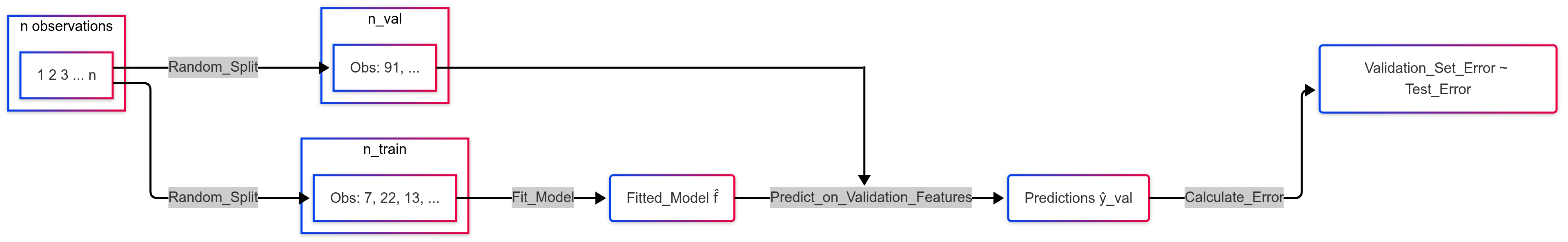
The Validation Set Approach
Concept: The simplest CV strategy.
Process:
Randomly divide the available dataset (size \(n\)) into two parts:
A training set (e.g., containing \(n_{train}\) observations).
A validation set or hold-out set (containing \(n_{val} = n - n_{train}\) observations). Typically a 70/30 or 80/20 split.
Fit the model only on the training set.
Use the fitted model to predict responses for the observations in the validation set.
Calculate the error (e.g., MSE or error rate) on the validation set. This is the validation set error, used as an estimate of the test error.
Validation Set Approach: Diagram
Let a dataset with size \(n = 100\), so an example of diagram is:
Validation Set Approach: R Example
Goal: Estimate test MSE for predicting mpg using polynomial functions of horsepower.
library(dplyr)# Use Auto datasetAuto <- ISLR::Auton <-nrow(Auto)print(paste("Sample size is:",n))# Set seed for reproducibilityset.seed(2)# Create a split: ~70% training, ~30% validationtrain_idx <-sample(n, round(.7*n), replace = F)train_dt <- Auto[train_idx,]test_dt <- Auto[-train_idx,] # Validation set contains observations NOT in train_idxprint(paste("Sample Train set is:", nrow(train_dt)))print(paste("Sample Test set is:", nrow(test_dt)))
[1] "Sample size is: 392"
[1] "Sample Train set is: 274"
[1] "Sample Test set is: 118"
Interpretation (for seed=2): The quadratic model seems best based on this single split, as it has the lowest estimated test MSE.
Validation Set Approach: Drawbacks
High Variability: The estimate of the test error can be highly variable. It strongly depends on which observations happen to end up in the training set versus the validation set.
Running the process again with a different random split will likely yield a different test error estimate and potentially suggest a different “best” model.
Overestimation of Test Error: The model is fit on only a subset of the data (e.g., 70% or 80%). Statistical methods tend to perform worse when trained on fewer observations. Therefore, the validation set error rate might overestimate the test error rate that would be obtained if the model were fit on the entire dataset.
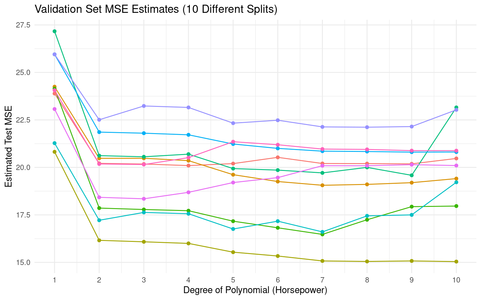
Validation Set Approach:
Variability Example
Let’s repeat the process 10 times with different random splits.
n_repeats <-10mse_results <-matrix(NA, nrow = n_repeats, ncol =10) # Store MSEs for degrees 1-10for (rep in1:n_repeats) {set.seed(rep +10) # Different seed each time train_idx_rep <-sample(n, round(.7*n), replace = F) train_dt <- Auto[train_idx_rep,] test_dt <- Auto[-train_idx_rep,] # Validation set contains observations NOT in train_idxfor (degree in1:10) { lm_fit_rep <-lm(mpg ~poly(horsepower, degree), data = train_dt) pred_rep <-predict(lm_fit_rep, test_dt) mse_results[rep, degree] <-mean((test_dt$mpg - pred_rep)^2) }}# DataFrame with MSEmse_df_long <-as.data.frame(mse_results)names(mse_df_long) <-1:10mse_df_long$Repeat <-1:n_repeatsmse_df_long <- tidyr::pivot_longer(mse_df_long, cols =-Repeat, names_to ="Degree", values_to ="MSE")mse_df_long$Degree <-as.integer(mse_df_long$Degree)
Observation: While all curves suggest quadratic is much better than linear, the exact minimum MSE and the benefit of higher orders vary considerably between splits.
The dataset for CV
Train, Validation, and Test Sets
From this point forward, we will work with the dataset split into three distinct parts, each with a specific role in the Statistical Machine Learning workflow:
Training - The portion of the data used to train the model — this is where the model learns patterns and relationships.
Validation - Used to evaluate the model after training and during the tuning process. Helps in selecting hyperparameters and avoiding overfitting.
Test - Reserved for the final evaluation of the model, providing an unbiased estimate of its real-world performance.
This structure helps ensure that the model generalizes well to unseen data.
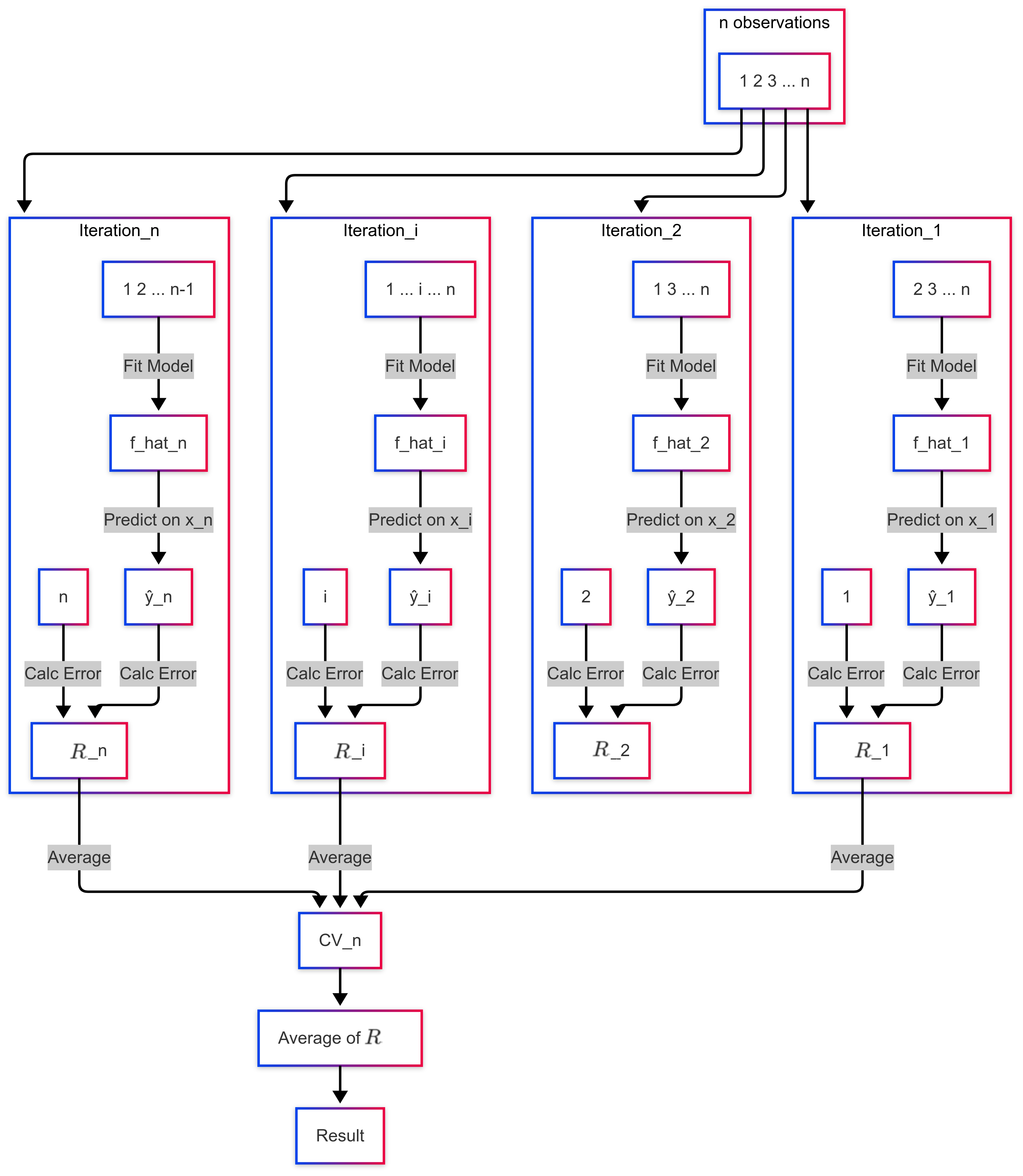
Leave-One-Out Cross-Validation
(LOOCV)
Concept: Addresses the drawbacks of the validation set approach.
Process:Only training dataset
Divide the data (\(n\) observations) into:
A validation set containing only one observation \((\dot{\mathbf{x}}_i, y_i)\).
A training set containing the remaining\(n-1\) observations.
Fit the model on the \(n-1\) training observations.
Make a prediction \(\hat{y}_i\) for the single held-out observation using its feature value \(\dot{\mathbf{x}}_i\).
Calculate the error for this observation with a risk function
\(R_i(\hat{y}_i)\)
Repeat this process \(n\) times, holding out each observation \(i=1, ..., n\) exactly once.
The LOOCV estimate of the test error is the average of these \(n\) individual errors: \[ CV_{(n)} = \frac{1}{n} \sum_{i=1}^n R_i \]
LOOCV: Diagram
Let a dataset with size \(n\), an example of LOOCV diagram is:
LOOCV: Advantages
Less Bias: The model is trained on \(n-1\) observations in each iteration, which is almost the entire dataset. This means the LOOCV estimate of test error tends to be less biased than the validation set estimate. It’s less likely to overestimate the true test error.
No Randomness: Unlike the validation set approach, LOOCV produces the same result every time it’s run on the same dataset. There’s no random splitting involved in the procedure itself (only in how the original data might have been collected). This makes results reproducible.
LOOCV: Disadvantages
Computationally Expensive: The model must be fit \(n\) times. This can be very slow if \(n\) is large or if the model itself takes a long time to fit.
(Exception: A shortcut exists for linear models fit by least squares, making it as fast as a single fit!)
2. Higher Variance (Potentially): While less biased, LOOCV estimates can sometimes have higher variance than other methods like k-fold CV. We are averaging the outputs of \(n\) models that are highly correlated (trained on almost identical datasets). Averaging highly correlated quantities yields an average with higher variance compared to averaging less correlated quantities.
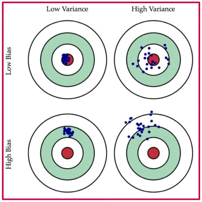
Trade-off: Bias and Variance
\(k\)-Fold Cross-Validation
Concept: An alternative to LOOCV that tries to balance bias, variance, and computation time.
\(k\)-Fold Cross-Validation
Concept: An alternative to LOOCV that tries to balance bias, variance, and computation time.
Process:Only training dataset
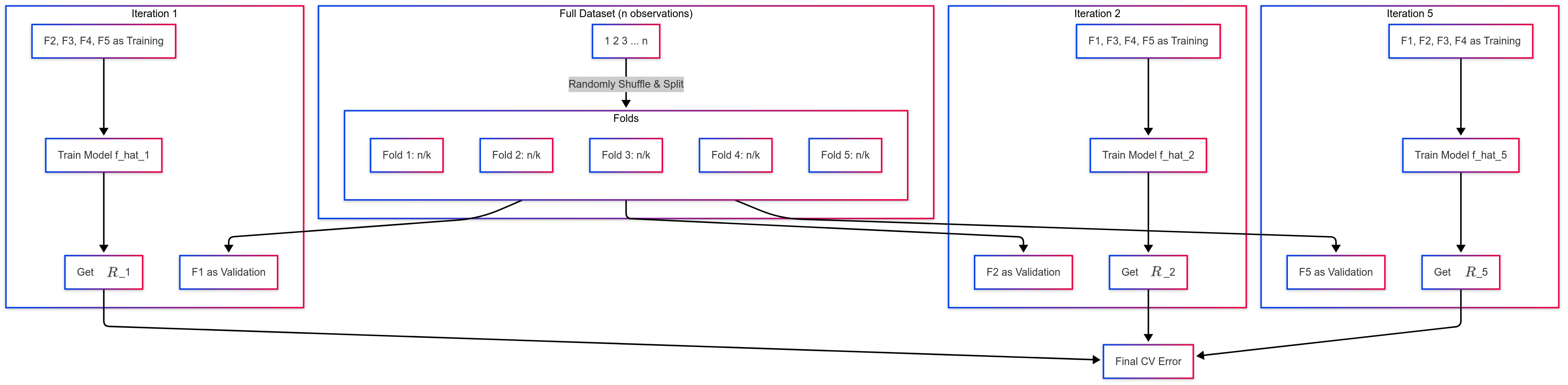
Randomly divide the set of \(n\) observations into \(k\) groups (or folds) of approximately equal size (typically \(k=5\) or \(k=10\)).
For each fold \(j = 1, ..., k\):
Treat fold \(j\) as the validation set.
Fit the model on the remaining \(k-1\) folds (the training set).
Compute the error (\(R_j\)) on the held-out fold \(j\), as
\[R_j(\hat{\mathbf{y}}_j),\]
where \(\hat{\mathbf{y}}_j\) has \(\left\lfloor \frac{n}{k}\right\rfloor\) observations.
The k-fold CV estimate of the test error is the average of these \(k\) errors: \[ CV_{(k)} = \frac{1}{k} \sum_{j=1}^k R_j(\hat{\mathbf{y}}_j) \]
Note: LOOCV is the special case where \(k=n\).
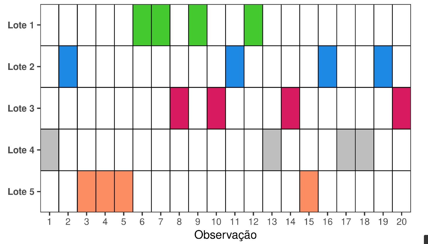
\(k\)-Fold CV: Diagram (k=5)
Let a dataset with size \(n\), an example of \(k\)-fold diagram is:
\(k\)-Fold CV: Advantages over LOOCV
Computational Efficiency: Requires fitting the model only \(k\) times (e.g., 10 times for 10-fold CV) instead of \(n\) times. This is a significant advantage when \(n\) is large and the fitting process is slow (and the LOOCV shortcut doesn’t apply).
Lower Variance (Often): Compared to LOOCV, k-fold CV often provides a test error estimate with lower variance. The \(k\) models being averaged are trained on less overlapping datasets compared to the \(n\) models in LOOCV. Averaging less correlated estimates tends to reduce variance more effectively.
Bias: k-fold CV generally has slightly more bias than LOOCV because the models are trained on \((k-1)/k\) of the data (e.g., 90% for k=10) instead of \((n-1)/n\). However, this bias is often considered a reasonable trade-off for the reduction in variance and computation time.
Bias-Variance:
Trade-off for \(k\)-Fold CV
Choice of k: Affects the bias-variance trade-off for the test error estimate.
Large k (approaching n, like LOOCV):
Lower Bias: Training sets are almost the full size \(n\).
Higher Variance: Models are trained on highly overlapping data, leading to correlated outputs whose average has high variance.
Computationally Expensive.
Small k (e.g., k=2 or k=3):
Higher Bias: Training sets are significantly smaller than \(n\).
Lower Variance: Models are trained on less overlapping data.
Computationally Cheaper.
Common Choice (k=5 or k=10): Empirically found to provide a good balance. Test error estimates suffer neither from excessively high bias nor very high variance.
\(k\)-Fold CV: R Example - \(k\)=10
Using boot::cv.glm() with the K argument.
# Set seed because the fold assignments are randomset.seed(17) cv_error_k10 <-rep(0, 10) # Store 10-fold CV errors# Loop through polynomial degreesfor (degree in1:10) { glm_fit <-glm(mpg ~poly(horsepower, degree), data = Auto)# Perform 10-fold CV using cv.glm with K=10 cv_results_k10 <-cv.glm(Auto, glm_fit, K =10) cv_error_k10[degree] <- cv_results_k10$delta[1] # delta[1] is the raw k-fold estimate}# Display resultsk10_results_df <-data.frame(Degree =1:10, K10_CV_MSE = cv_error_k10)print(k10_results_df |>head(), row.names =FALSE)
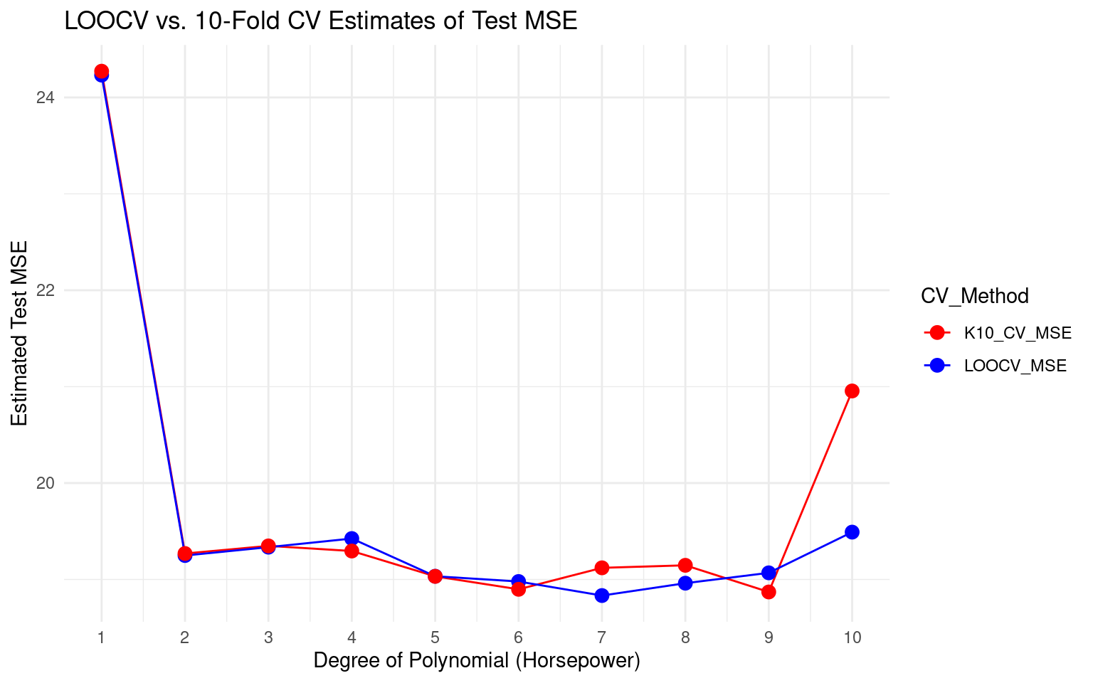
Let’s plot the LOOCV and 10-Fold CV estimates together.
Observation: The curves are quite similar, both suggesting the quadratic model is optimal. 10-fold CV is computationally much faster if the shortcut isn’t available.
CV for Classification Problems
CV works similarly for classification where \(Y\) is qualitative.
Key Difference: Instead of using MSE to quantify error, we typically use the number of misclassified observations (or the misclassification rate).
Validation Set Error Rate: Proportion of validation observations misclassified.
LOOCV Error Rate:\[ CV_{(n)} = \frac{1}{n} \sum_{i=1}^n I(y_i \neq \hat{y}_i) \] (\(I(\cdot)\) is an indicator function: 1 if true, 0 if false. \(\hat{y}_i\) is the prediction for the \(i\)-th observation when it was held out).
CV for Classification Problems
CV works similarly for classification where \(Y\) is qualitative.
Key Difference: Instead of using MSE to quantify error, we typically use the number of misclassified observations (or the misclassification rate).
Validation Set Error Rate: Proportion of validation observations misclassified.
k-Fold CV Error Rate:\[ CV_{(k)} = \frac{1}{k} \sum_{i=1}^k \left( \frac{1}{t_k} \sum_{j=1}^{t_k} I(y_j \neq \hat{y}_j) \right)\] (\(I(\cdot)\) is an indicator function: 1 if true, 0 if false. \(\hat{y}_j\) is the prediction for the \(j\)-th observation and \(k\)-th fold, and \(t_k\) is the number of observations in the \(k\)-th fold).
CV for Classification Problems
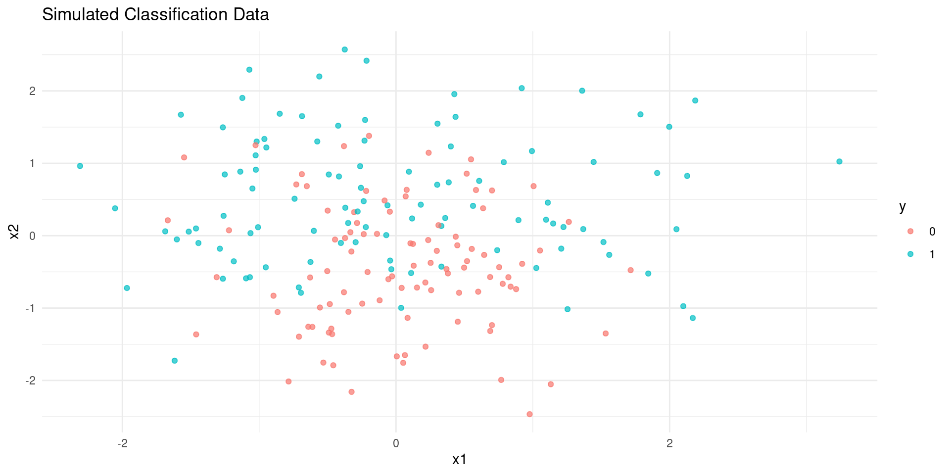
Simulated Data and Logistic Regression
We’ll fit logistic regression with polynomial predictors and use 10-fold CV to select the polynomial degree. We need to generate 2D data for a binary classification task.
# Generate simulated data (similar spirit to Fig 2.13)set.seed(123)n_sim <-200x1 <-rnorm(n_sim)x2 <-rnorm(n_sim)# Create a non-linear boundary based on x1^2 + x2 - 2prob <-1/ (1+exp(-(x1^2+ x2 -1))) # Example boundarysummary(prob)y <-rbinom(n_sim, 1, prob)sim_data <-data.frame(x1 = x1, x2 = x2, y =factor(y))# Plot the simulated datalibrary(ggplot2)p <-ggplot(sim_data, aes(x = x1, y = x2, color = y)) +geom_point(alpha =0.7) +labs(title ="Simulated Classification Data") +theme_minimal()
   Min. 1st Qu.  Median    Mean 3rd Qu.    Max.
0.04512 0.23402 0.40139 0.46038 0.67066 0.99997
CV for Classification Problems
Simulated Data and Logistic Regression
plot(p)
CV for Classification Problems
Simulated Data and Logistic Regression
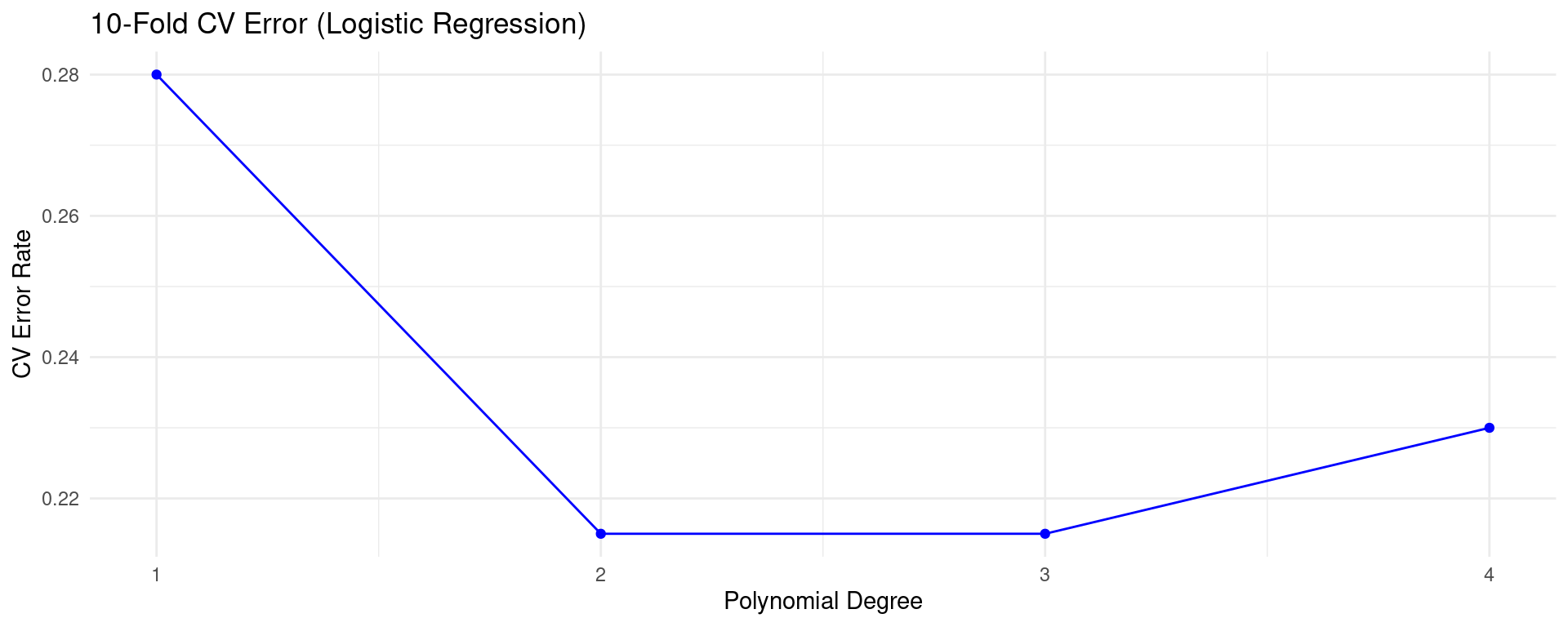
Use 10-fold CV to estimate test error rate for logistic regression with polynomials of \(X1\) and \(X2\). Note: cv.glm doesn’t directly calculate misclassification rate. We need a custom cost function.
# Cost function for misclassification rate with cv.glmcost_misclass <-function(r, pi) {# r: actual response (0 or 1)# pi: predicted probability# Convert probabilities to class predictions (threshold 0.5) pred_class <-ifelse(pi >0.5, 1, 0)# Calculate misclassification ratemean(r != pred_class)}set.seed(42)k_folds <-10cv_error_logit <-rep(NA, 4) # Test degrees 1 to 4for (degree in1:4) {# Formula: y ~ poly(x1, degree) + poly(x2, degree) # Note: Interaction terms might also be considered fit_formula <-as.formula(paste("y ~ poly(x1, ", degree, ") + poly(x2, ", degree, ")")) glm_fit_class <-glm(fit_formula, data = sim_data, family = binomial)# Use cv.glm with custom cost function# Important: cv.glm needs numeric response 0/1 for binomial sim_data_numeric <- sim_data sim_data_numeric$y <-as.numeric(sim_data_numeric$y) -1# Convert factor to 0/1 cv_res_class <-cv.glm(sim_data_numeric, glm_fit_class, cost = cost_misclass, K = k_folds) cv_error_logit[degree] <- cv_res_class$delta[1] }logit_cv_results <-data.frame(Degree =1:4, CV_ErrorRate = cv_error_logit)print(logit_cv_results)
Use 10-fold CV to estimate test error rate for logistic regression with polynomials of \(X1\) and \(X2\). Note: cv.glm doesn’t directly calculate misclassification rate. We need a custom cost function.
Observation: CV helps find the optimal flexibility (Polynomial Degree) that minimizes the estimated test error.
Handling Imbalanced Data: Resampling Techniques
Strategies for Balancing Datasets in Statistical Machine Learning
What is Data Imbalance?
Occurs when classes in a classification problem are not represented equally.
One class (the majority class) dominates the dataset, while others (the minority class(es)) are significantly underrepresented.
Example:
Fraud detection (1% fraud, 99% non-fraud),
medical diagnosis (rare diseases), anomaly detection.
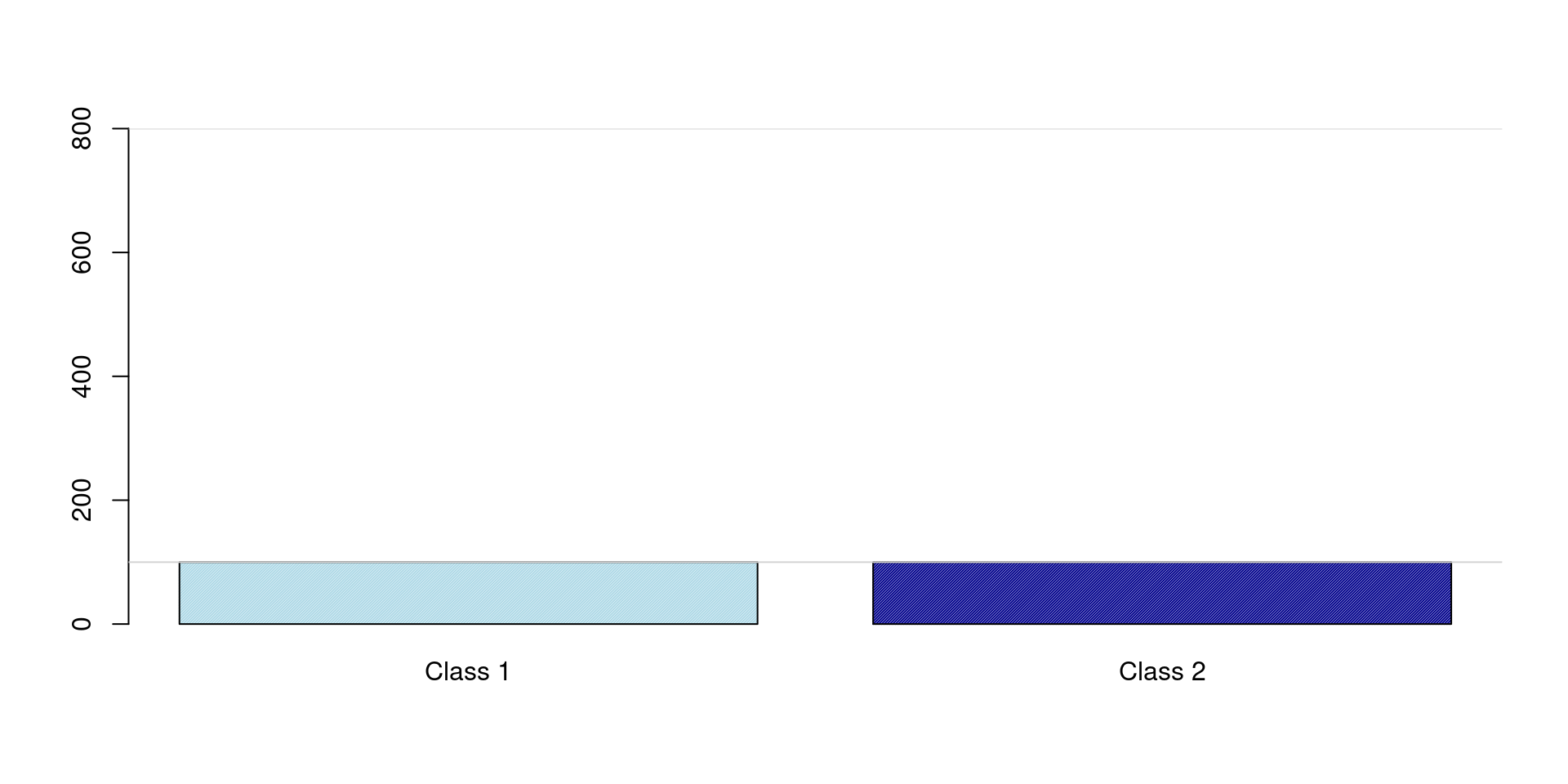
Class Distribution
Example:
Class A:
950 samples (Majority)
Class B:
50 samples (Minority)
Total (n):
1000
Why is Imbalance a Problem?
Model Bias: Standard algorithms aim to minimize overall error (or maximize accuracy). They often achieve this by focusing on the majority class, potentially ignoring the minority class entirely.
Poor Minority Class Performance: The model may perform poorly in identifying minority class instances, which are often the cases of interest (e.g., detecting fraud).
Misleading Evaluation: Standard metrics like accuracy can be deceptive. A model predicting the majority class every time can achieve high accuracy but be useless in practice.
Example: Predicting “non-fraud” 100% of the time gives 99% accuracy in the previous example, but fails to catch any fraud.
Balancing Techniques Overview
Goal: Adjust the class distribution of the training data (\(\dot{\mathbf{X}}_{train}, \dot{\mathbf{y}}_{train}\)) to help the model learn patterns from the minority class.
Main Approaches:
Undersampling: Remove samples from the majority class.
Oversampling: Add samples to the minority class.
Synthetic Data Generation: Create new artificial samples for the minority class (e.g., SMOTE).
Important: Apply these techniques only to the training data, after splitting your original dataset.
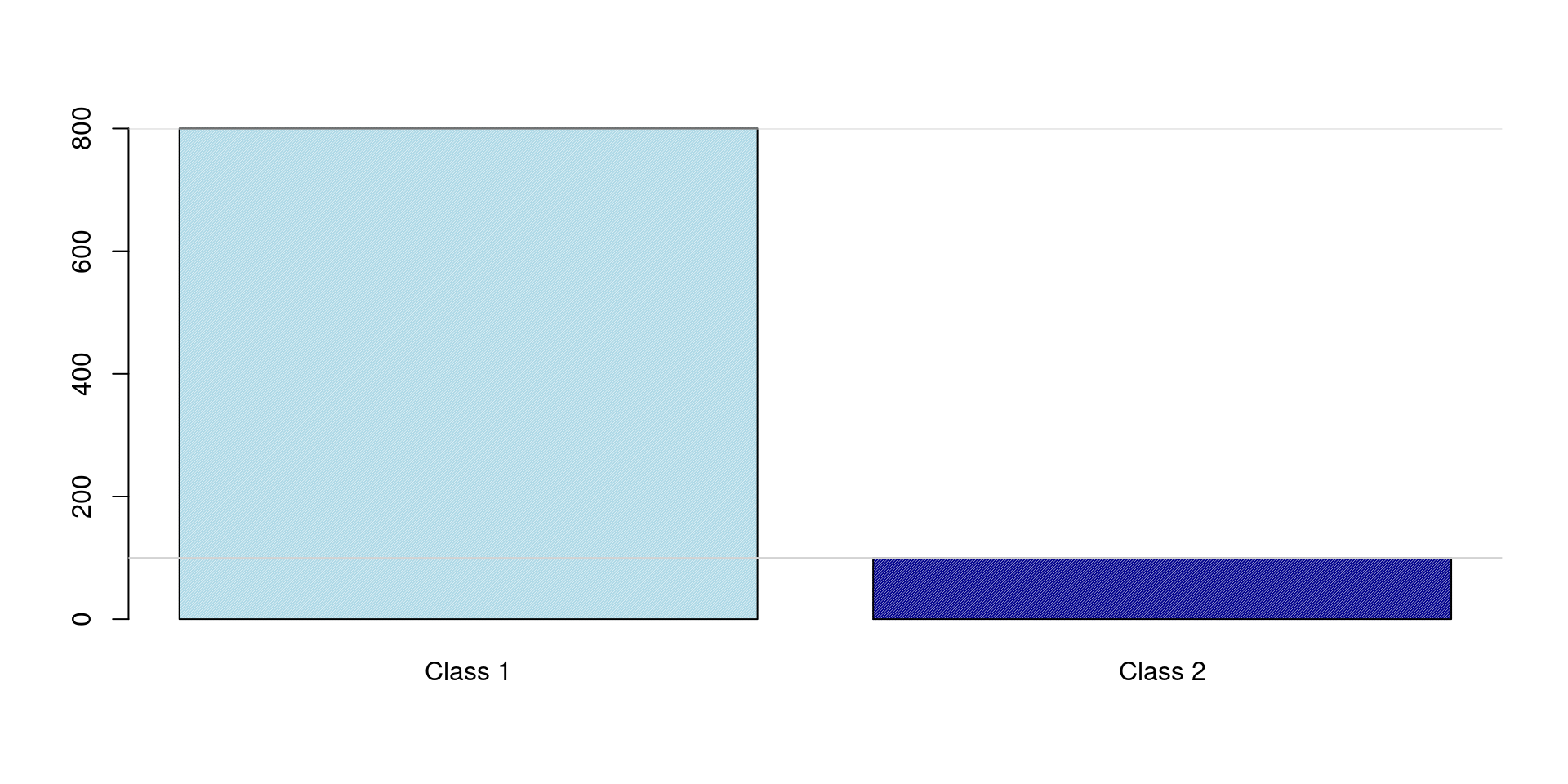
Undersampling: Concept
Idea: Reduce the size of the majority class to balance it with the minority class.
Mechanism: Discard instances (\(\dot{\mathbf{x}}_i, y_i\)) belonging to the majority class.
Result: A smaller, more balanced training dataset.
Undersampling: Concept
Undersampling: Pros & Cons
Pros:
Can significantly reduce the size of the training dataset (\(n_{train}\) decreases).
May lead to faster model training times.
Can help when the majority class has redundant information.
Cons:
Potential Information Loss: Removing instances might discard valuable information about the majority class boundary, potentially harming model performance.
May not be suitable if the initial dataset size (\(n\)) is small.
Random Undersampling
Simplest form of undersampling.
Method: Randomly select and remove instances from the majority class until the desired class balance is reached (often 1:1 with the minority class).
Implementation: Easy to implement but prone to removing informative instances purely by chance.
Random Undersampling - RUS
R Example
# Required libraries# install.packages("caret") # or install.packages("themis") for tidymodelslibrary(caret)library(dplyr)# --- Create Sample Imbalanced Data ---set.seed(123)n_maj <-950n_min <-50p_features <-5X_maj <-matrix(rnorm(n_maj * p_features, mean =0), ncol = p_features)X_min <-matrix(rnorm(n_min * p_features, mean =2), ncol = p_features) # Separable# Combine features (X) and labels (y)dot_X <-as.data.frame(rbind(X_maj, X_min))colnames(dot_X) <-paste0("V", 1:p_features)y <-factor(c(rep("Majority", n_maj), rep("Minority", n_min)))original_data <-bind_cols(dot_X, Class = y)cat("Original Class Distribution:\n")print(table(original_data$Class))# --- Apply Random Undersampling using caret::downSample ---# Note: Assumes data split into train/test already. Apply to train set.# Here, applying to 'original_data' for demonstration.set.seed(456)# downSample requires predictor matrix (dot_X) and outcome vector (y)undersampled_data <- caret::downSample(x = original_data[, -ncol(original_data)], # Features dot_Xy = original_data$Class, # Labels ylist =FALSE, # Return data frameyname ="Class")cat("\nUndersampled Class Distribution:\n")print(table(undersampled_data$Class))
Random Undersampling - RUS
Python Example
# Required libraries# pip install scikit-learn imbalanced-learnimport numpy as npimport pandas as pdfrom sklearn.datasets import make_classificationfrom imblearn.under_sampling import RandomUnderSamplerfrom collections import Counter# --- Create Sample Imbalanced Data ---# Generating feature matrix (X) and label vector (y)dot_X, y = make_classification(n_samples=1000, n_features=5, n_informative=3, n_redundant=0, n_repeated=0, n_classes=2, weights=[0.95, 0.05], flip_y=0, random_state=123)print(f"Original dataset shape: {dot_X.shape}")print(f"Original class distribution: {Counter(y)}") # 0: Majority, 1: Minority# --- Apply Random Undersampling using imblearn ---# Note: Apply ONLY to training data after train/test split.rus = RandomUnderSampler(sampling_strategy='auto', # Balances to minority class count random_state=456)dot_X_resampled, y_resampled = rus.fit_resample(dot_X, y)print(f"\nResampled dataset shape: {dot_X_resampled.shape}")print(f"Resampled class distribution: {Counter(y_resampled)}")
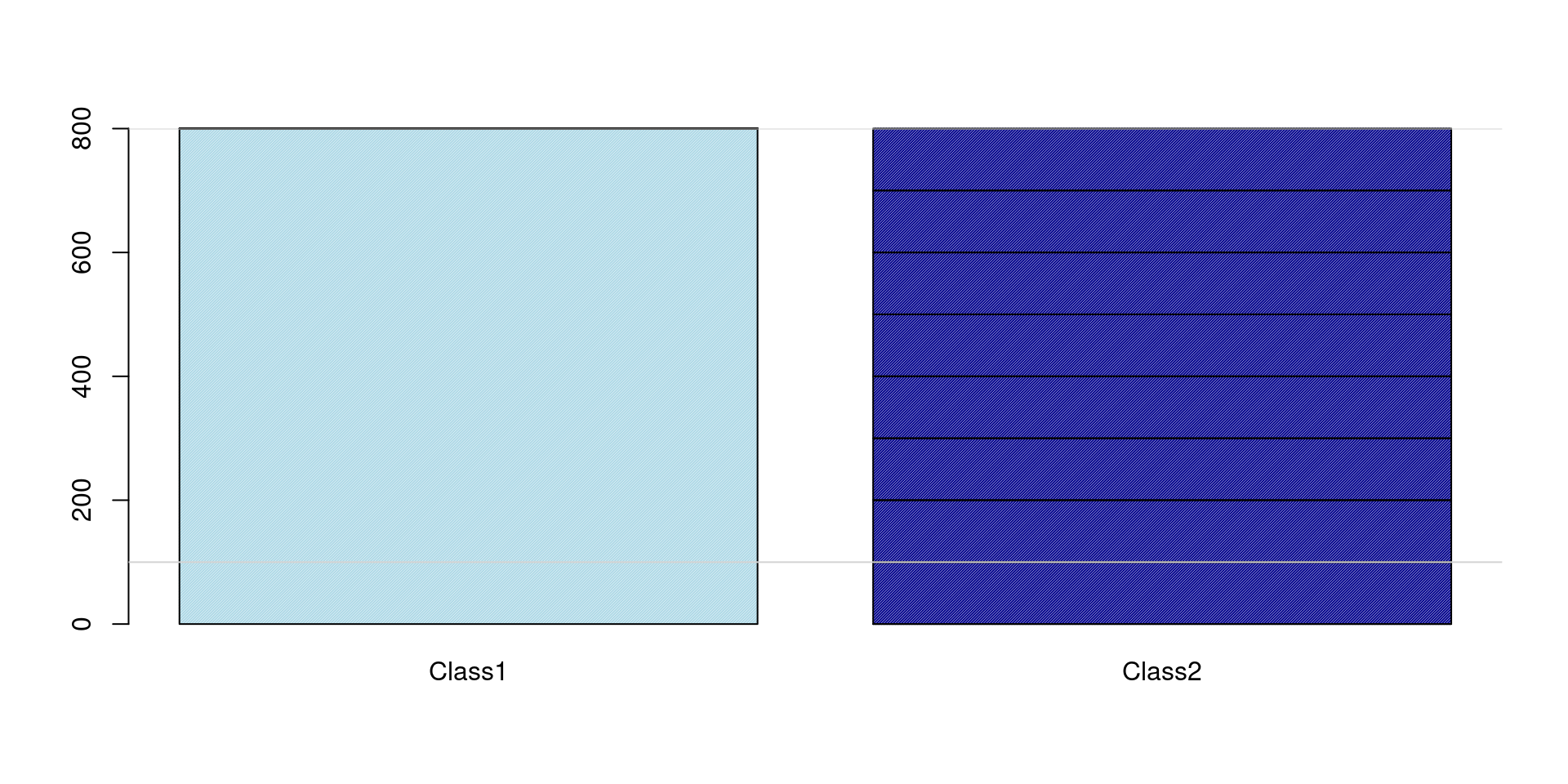
Oversampling: Concept
Idea: Increase the size of the minority class to balance it with the majority class.
Mechanism: Add instances (\(\dot{\mathbf{x}}_i, y_i\)) belonging to the minority class.
Result: A larger, more balanced training dataset.
Oversampling: Concept
Oversampling: Pros & Cons
Pros:
No Information Loss: Unlike undersampling, no instances from the original dataset are discarded. All original information is retained.
Often performs well when the minority class contains important, unique patterns.
Cons:
Increased Training Time: The size of the training dataset (\(n_{train}\)) increases, potentially leading to longer model training.
Risk of Overfitting (especially with Random Oversampling): Making exact copies of minority instances can lead the model to learn specific examples rather than general patterns.
Random Oversampling
Simplest form of oversampling.
Method: Randomly select instances from the minority class, with replacement, and add these copies to the training dataset until the desired class balance is reached.
Implementation: Easy to implement but prone to overfitting, as the model might see the exact same minority instance multiple times.
Random Oversampling - ROS
R Example
# Required librarieslibrary(caret)library(dplyr)# --- Create Sample Imbalanced Data ---set.seed(456)n_maj <-950n_min <-50p_features <-5X_maj <-matrix(rnorm(n_maj * p_features, mean =0), ncol = p_features)X_min <-matrix(rnorm(n_min * p_features, mean =2), ncol = p_features) # Separable# Combine features (X) and labels (y)dot_X <-as.data.frame(rbind(X_maj, X_min))colnames(dot_X) <-paste0("V", 1:p_features)y <-factor(c(rep("Majority", n_maj), rep("Minority", n_min)))original_data <-bind_cols(dot_X, Class = y)# --- Use the same Sample Imbalanced Data ---cat("Original Class Distribution:\n")print(table(original_data$Class))# --- Apply Random Oversampling using caret::upSample ---set.seed(789)# upSample requires predictor matrix (X) and outcome vector (y)oversampled_data <- caret::upSample(x = original_data[, -ncol(original_data)], # Features Xy = original_data$Class, # Labels ylist =FALSE, # Return data frameyname ="Class")cat("\nOversampled Class Distribution:\n")print(table(oversampled_data$Class))cat(paste("\nTotal samples after oversampling:", nrow(oversampled_data), "\n"))
Random Oversampling - ROS
Python Example
# Required libraries (reuse from RUS example)import numpy as npfrom sklearn.datasets import make_classificationfrom imblearn.over_sampling import RandomOverSamplerfrom collections import Counter# --- Create Sample Imbalanced Data ---# Generating feature matrix (X) and label vector (y)dot_X, y = make_classification(n_samples=1000, n_features=5, n_informative=3, n_redundant=0, n_repeated=0, n_classes=2, weights=[0.95, 0.05], flip_y=0, random_state=456)print(f"Original dataset shape: {dot_X.shape}")print(f"Original class distribution: {Counter(y)}") # 0: Majority, 1: Minority# --- Apply Random Oversampling using imblearn ---ros = RandomOverSampler(sampling_strategy='auto', # Balances to majority class count random_state=789)dot_X_resampled, y_resampled = ros.fit_resample(dot_X, y)print(f"\nResampled dataset shape: {dot_X_resampled.shape}")print(f"Resampled class distribution: {Counter(y_resampled)}")
SMOTE
Synthetic Minority Over-sampling Technique
Problem with Oversample: Duplicating samples can lead to overfitting.
SMOTE Idea: Generate new, synthetic minority class samples instead of just copying existing ones.
How it Works (Simplified):
For each minority instance (\(\dot{\mathbf{x}}_i\)).
Find its k nearest neighbors (\(\dot{\mathbf{x}}_{zi}\)) that are also in the minority class.
Randomly choose one of these neighbors (\(\dot{\mathbf{x}}_{zi}\)).
Create a synthetic sample (\(\dot{\mathbf{x}}_{new}\)) along the line segment connecting \(\dot{\mathbf{x}}_i\) and \(\dot{\mathbf{x}}_{zi}\): \(\dot{\mathbf{x}}_{new} = \dot{\mathbf{x}}_i + \lambda (\dot{\mathbf{x}}_{zi} - \dot{\mathbf{x}}_i)\), where \(\lambda\) is a random number in \([0, 1]\).
Result: Expands the decision region of the minority class without exact duplication.
SMOTE: Pros & Cons
Pros:
Mitigates Overfitting: Creates new synthetic samples, reducing the risk associated with simple duplication (ROS).
No Information Loss: Retains all original data points.
Often leads to better generalization compared to ROS.
Cons:
Can Create Noise: If minority/majority classes overlap significantly, SMOTE might generate synthetic samples in ambiguous regions or even within the majority class space (“bridging”).
Not Effective for High Dimensionality: The “nearest neighbor” concept becomes less meaningful in very high-dimensional spaces (\(p\) is large) - Curse of Dimensionality.
Parameter sensitive (choice of \(k\) neighbors).
SMOTE
R Example
# Required librarylibrary(themis) # Using themis for tidymodels integrationlibrary(recipes)library(dplyr)# --- Create Sample Imbalanced Data ---set.seed(789)n_maj <-950n_min <-50p_features <-5X_maj <-matrix(rnorm(n_maj * p_features, mean =0), ncol = p_features)X_min <-matrix(rnorm(n_min * p_features, mean =2), ncol = p_features) # Separable# Combine features (X) and labels (y)dot_X <-as.data.frame(rbind(X_maj, X_min))colnames(dot_X) <-paste0("V", 1:p_features)y <-factor(c(rep("Majority", n_maj), rep("Minority", n_min)))original_data <-bind_cols(dot_X, Class = y)cat("Original Class Distribution:\n")print(table(original_data$Class))summary(original_data[original_data$Class =="Majority",])summary(original_data[original_data$Class =="Minority",])# --- Apply SMOTE using themis::step_smote within a recipe ---# This is the modern 'tidymodels' waysmote_recipe <-recipe(Class ~ ., data = original_data) |># Target ratio: 'over_ratio = 1' means minority class size = majority class sizestep_smote(Class, over_ratio =1, neighbors =5, seed =1011)# Prepare and apply the recipe# 'prep' estimates parameters (like neighbors), 'bake' applies the stepssmote_prep <-prep(smote_recipe)smoted_data <-bake(smote_prep, new_data =NULL) # Apply to original datacat("\nSMOTE'd Class Distribution:\n")print(table(smoted_data$Class))cat(paste("\nTotal samples after SMOTE:", nrow(smoted_data), "\n"))summary(smoted_data[smoted_data$Class =="Minority",])
SMOTE
Python Example
# Required libraries (reuse from previous examples)import numpy as npfrom sklearn.datasets import make_classificationfrom imblearn.over_sampling import SMOTEfrom collections import Counter# --- Create Sample Imbalanced Data ---# Generating feature matrix (X) and label vector (y)dot_X, y = make_classification(n_samples=1000, n_features=5, n_informative=3, n_redundant=0, n_repeated=0, n_classes=2, weights=[0.95, 0.05], flip_y=0, random_state=789)print(f"Original dataset shape: {dot_X.shape}")print(f"Original class distribution: {Counter(y)}") # 0: Majority, 1: Minority# --- Apply SMOTE using imblearn ---# sampling_strategy='auto' typically means balancing to the majority class count# k_neighbors is the number of neighbors used (default is 5)smt = SMOTE(sampling_strategy='auto', k_neighbors=5, random_state=1011)dot_X_resampled, y_resampled = smt.fit_resample(dot_X, y)print(f"\nResampled dataset shape: {dot_X_resampled.shape}")print(f"Resampled class distribution: {Counter(y_resampled)}")
Crucial Workflow: Splitting First!
NEVER apply balancing techniques before splitting your data into training and testing sets.
Why? Applying balancing to the entire dataset causes data leakage.
Undersampling: Test set might lose representative majority samples.
Oversampling/SMOTE: Synthetic samples based on the entire dataset (including future test points) might appear in the training set, and copies/neighbors of test points might appear in the training set. This gives an overly optimistic evaluation.
Crucial Workflow: Splitting First!
Correct Workflow:
Split Data: Divide original (\(\dot{\mathbf{X}}, \dot{\mathbf{y}}\)) into Training (\(\dot{\mathbf{X}}_{train}, \dot{\mathbf{y}}_{train}\)) and Testing (\(\dot{\mathbf{X}}_{test}, \dot{\mathbf{y}}_{test}\)).
Apply Balancing (Train Only): Use RUS, ROS, SMOTE, etc., only on (\(\dot{\mathbf{X}}_{train}, \dot{\mathbf{y}}_{train}\)) to get (\(\dot{\mathbf{X}}_{train\_bal}, \dot{\mathbf{y}}_{train\_bal}\)).
Train Model: Train your classifier on the balanced training data (\(\dot{\mathbf{X}}_{train\_bal}, \dot{\mathbf{y}}_{train\_bal}\)).
Evaluate Model: Evaluate the trained model on the original, unbalanced test set (\(\dot{\mathbf{X}}_{test}, \dot{\mathbf{y}}_{test}\)) using appropriate metrics1.
Extra: Critical Difference
Comparing Multiple Algorithms
Challenge: We often develop multiple models (\(M_1, M_2, ..., M_m\)) or configure algorithms with different parameters. How do we rigorously compare their performance?
Common Scenario: Evaluating these \(m\) models across \(k\) different datasets or \(k\) cross-validation folds from a single dataset.
Problem with Simple Averaging: Just averaging a metric (like AUC, accuracy, error rate) across datasets/folds can be misleading. A model might perform exceptionally well on easy datasets/folds but poorly on hard ones, skewing the average. We need to know if performance differences are statistically significant.
Goal: Determine if observed differences in performance are statistically significant or just due to chance variability across the \(k\) datasets/folds.
Statistical Comparison Framework
Approach: Use statistical tests designed for comparing multiple measurements (models) across multiple groups (datasets/folds).
Workflow:
Omnibus Test1: First, check if there are any statistically significant differences among the models’ performances overall.
Common Choice: Friedman Test (non-parametric).
Post-Hoc Test: If the omnibus test finds significant differences, perform pairwise comparisons to identify which specific models differ significantly from each other.
Common Choice: Nemenyi Test (specifically designed as a post-hoc for Friedman).
Visualization: Summarize the results of the post-hoc test using a Critical Difference Diagram.
Step 1: Friedman Test
Purpose: A non-parametric statistical test to detect differences in treatments (our \(m\) models) across multiple test attempts (\(k\) datasets/folds), using ranks.
Analogy: Similar to a repeated-measures ANOVA, but works on ranks, making it suitable when metric distributions aren’t normal.
Procedure:
For each dataset/fold \(D_i\) (\(i=1, ..., k\)), rank the \(m\) models based on their performance metric (e.g., rank 1 for lowest error, highest AUC). Handle ties by assigning average ranks.
Calculate the average rank \(R_j\) for each model \(M_j\) across all \(k\) datasets/folds: \(R_j = \frac{1}{k} \sum_{i=1}^{k} rank(\dot{m}_{ij})\), where \(\dot{m}_{ij}\) is the performance of model \(j\) on dataset/fold \(i\).
The test statistic evaluates if the observed average ranks \(R_j\) are significantly different from what’s expected if all models performed equally (i.e., all \(R_j\) were the same).
Step 1: Friedman Test
Hypotheses:
\(H_0\): The average ranks of all \(m\) models are equal (no difference in performance).
\(H_1\): At least one model has a different average rank (performance differs).
Outcome: A p-value. If p < \(\alpha\) (e.g., 0.05), we reject \(H_0\) and conclude there are significant differences, justifying post-hoc analysis.
Step 2: Nemenyi Post-Hoc Test
Purpose: If the Friedman test is significant, the Nemenyi test identifies which pairs of models \((M_j, M_{j'})\) (where \(j, j' \in \{1, ..., m\}\)) have statistically significant differences in their average ranks (\(R_j, R_{j'}\)).
Concept: Compares the absolute difference in average ranks \(|R_j - R_{j'}|\) against a threshold called the Critical Difference (CD).
Step 2: Nemenyi Post-Hoc Test
Critical Difference (CD): The minimum difference in average ranks required to declare a statistically significant difference at a chosen significance level \(\alpha\).
\(CD = q_{\alpha} \sqrt{\frac{m(m+1)}{6k}}\)
\(q_{\alpha}\) is the critical value from the Studentized range statistic distribution for \(m\) groups (models) and infinite degrees of freedom (as Nemenyi is based on ranks)1. > qtukey(0.95, 4, Inf) # para alpha = 0.05 e m = 4
Decision Rule: Two models \(M_j\) and \(M_{j'}\) are considered significantly different if \(|R_j - R_{j'}| > CD\).
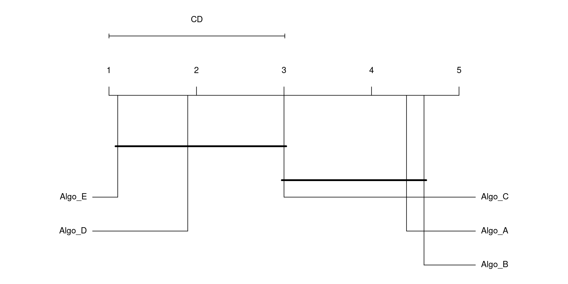
Visualizing Results
Critical Difference Diagram
Purpose: Provides a compact visual summary of the Nemenyi test results.
Construction:
A horizontal axis represents the average ranks (\(R_j\)). The \(m\) models are plotted along this axis according to their rank (lower ranks often plotted to the left, indicating better performance if using error rates).
A bar is drawn above the axis indicating the length of the Critical Difference (CD).
Key Feature: A thick horizontal line connects groups of models whose average ranks differ by less than the CD.
Interpretation: Any two models connected by the same horizontal bar are not statistically significantly different from each other (at the chosen \(\alpha\)). If two models are not connected by the same bar, their performance difference is statistically significant.
Critical Difference Diagram
R Example Setup
Required Library:scmamp (Statistical Comparison of Multiple Algorithms in Multiple Problems).
Input Data Format: A matrix perf_data where:
Rows represent datasets or folds (\(k\)).
Columns represent algorithms/models (\(m\)).
Values perf_data[i, j] contain the performance metric \(\dot{m}_{ij}\) of model \(j\) on dataset/fold \(i\).
Important: The ranking assumes lower values are better by default in scmamp. Use metrics like error rate or 1 - Accuracy, 1 - AUC.
Critical Difference Diagram
R Example Setup
Example Scenario: We compare \(m=5\) algorithms (Algo_A to Algo_E) across \(k=10\) datasets/folds, using their error rates.
# Install if needed: install.packages("scmamp")library(scmamp)# --- Create Sample Performance Data (ERROR RATES - lower is better) ---set.seed(123)m_models <-5# Number of models (m in our notation)k_datasets <-10# Number of datasets/folds (k in our notation)# Simulate error rates for m models across k datasets/foldsperf_data <-matrix(runif(m_models * k_datasets, min =0.5, max =0.7),nrow = k_datasets, ncol = m_models)# Let's make Algo_A generally better and Algo_E generally worseperf_data[, 1] <- perf_data[, 1] *0.3# Lower error for Algo_Aperf_data[, 2] <- perf_data[, 2] *0.3# Lower error for Algo_Aperf_data[, 3] <- perf_data[, 3] *0.4# Lower error for Algo_Aperf_data[, 5] <- perf_data[, 5] *1.2# Higher error for Algo_Ecolnames(perf_data) <-paste0("Algo_", LETTERS[1:m_models])rownames(perf_data) <-paste0("Dataset_or_Fold_", 1:k_datasets)
Function:scmamp::plotCD() performs the Friedman test, Nemenyi post-hoc test, and generates the diagram using the performance matrix.
# --- Generate the Critical Difference Diagram ---# Check Friedman test result (optional, plotCD does this internally)friedman_result <-friedmanTest(perf_data)print(paste("Friedman Test p-value:", friedman_result$p.value))
[1] "Friedman Test p-value: 1.51846285323387e-07"
# If p-value < alpha (e.g., 0.05), post-hoc comparison is meaningful.
Critical Difference Diagram
R Example Code and Plot
# Plot the CD diagram using Nemenyi test (default)# alpha: significance level# cex: text size scalingplotCD(results.matrix = perf_data, alpha =0.05, cex =0.9)
Summary & Interpretation
Critical Difference Diagrams provide a statistically sound and visually intuitive way to compare \(m\) classifiers across \(k\) datasets or folds.
They are based on ranking performance, followed by the Friedman test (to check for any overall difference) and the Nemenyi post-hoc test (for pairwise comparisons).
Reading the Diagram:
Models are ordered by average rank (lower rank = better performance if using error/loss).
Models connected by the same thick horizontal bar are not significantly different.
Models not connected by the same bar are significantly different.
Use Case: Helps identify the top-performing model(s) and group statistically equivalent models.
Summary & Interpretation
Caveats:
Requires sufficient datasets/folds (\(k\)) for reliable results (recommendations vary, often \(k > 10\)).
Sensitive to the chosen performance metric.
The Nemenyi test can be conservative; other post-hoc tests (e.g., Holm’s procedure) might offer more power.
References: Extras
Papers:
Chawla, N. V., Bowyer, K. W., Hall, L. O., & Kegelmeyer, W. P. (2002). SMOTE: Synthetic Minority Over-sampling Technique. Journal of Artificial Intelligence Research, 16, 321–357.
He, H., & Garcia, E. A. (2009). Learning from Imbalanced Data. IEEE Transactions on Knowledge and Data Engineering, 21(9), 1263–1284.
Popular Libraries:
Python:
imbalanced-learn (imblearn): Comprehensive library for resampling techniques. Integrates with scikit-learn. https://imbalanced-learn.org/
An Introduction to Statistical Learning: with Applications in R, James, G., Witten, D., Hastie, T. and Tibshirani, R., Springer, 2013, link: https://www.statlearning.com/.
Mathematics for Statistical Machine Learning, Deisenroth, M. P., Faisal. A. F., Ong, C. S., Cambridge University Press, 2020, link: https://mml-book.com.
References
Complementaries
An Introduction to Statistical Learning: with Applications in python, James, G., Witten, D., Hastie, T. and Tibshirani, R., Taylor, J., Springer, 2023, link: https://www.statlearning.com/.
Matrix Calculus (for Statistical Machine Learning and Beyond), Paige Bright, Alan Edelman, Steven G. Johnson, 2025, link: https://arxiv.org/abs/2501.14787.
Statistical Machine Learning Beyond Point Predictions: Uncertainty Quantification, Izibicki, R., 2025, link: https://rafaelizbicki.com/UQ4ML.pdf.