To motivate our study of statistical learning, let us begin with an illustrative example:
Suppose we are statistical consultants commissioned by a client to provide guidance on improving the sales of a specific product.
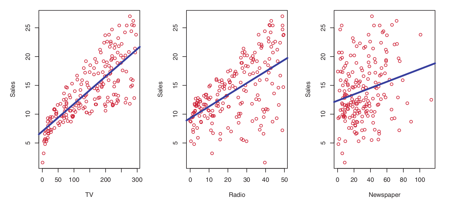
The Advertising dataset comprises the sales figures of this product across 200 distinct markets, alongside the advertising budgets allocated to each market across three different media channels: TV, radio, and newspaper.
The client cannot directly manipulate product sales; however, they can control advertising expenditures within each of these three media platforms.
Therefore, if we identify a significant association between advertising and sales, we can advise the client on budget adjustments to indirectly drive sales growth. In other words, our objective is to develop an accurate model capable of predicting sales based on expenditures across the three media outlets.
Statistical Learning?
To motivate our study of statistical learning, let us begin with an example:
In this context, the advertising budgets represent the input variables, whereas sales constitutes the output variable.
Input variables are generally denoted by the symbol \(X\), using subscripts to distinguish between them. Thus:
\(X_1\) may represent the TV budget;
\(X_2\) the radio budget; and
\(X_3\) the newspaper budget.
Input variables are known by various terms, such as predictors, independent variables, features, or occasionally simply variables.
The output variable—in this case, sales—is often referred to as the response, dependent variable, or label, and is typically represented by the symbol \(Y\).
Statistical Learning?
Statistical Learning?
Example 2:
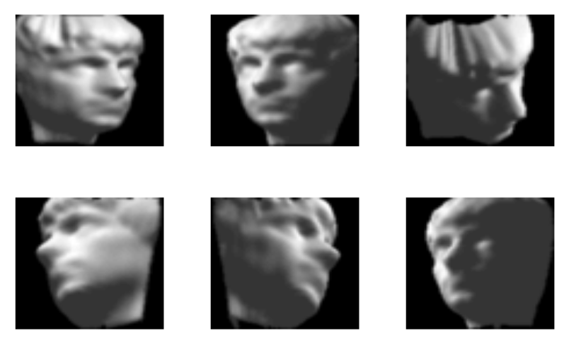
Isomap face data
Given a dataset of facial images, the objective is to determine the direction in which a person is looking based on a specific image of that individual.
One approach to this task involves developing a model that utilizes face images as input variables to predict the facial orientation as the response. Thus:
\(X_1\): facial image
and
\(Y\): facial orientation (pose direction)
Statistical Learning?
More generally, suppose we observe a quantitative response \(Y \in \mathbb{R}\) and \(p\) different predictors, \(X_1, X_2, \dots, X_p \in \mathbb{R}\).
We assume that there exists a relationship between \(Y\) and \(\mathbf{x} = (X_1, X_2, \dots, X_p)\), which can be expressed in a general form as:
\[
Y = f(\mathbf{x}) + \varepsilon,
\]
where \(\mathbf{x} \in \mathbb{R}^p\), \(f(\cdot)\) is a fixed but unknown function of \(X_1, \dots, X_p\), and \(\varepsilon\) is a random error term, which is independent of \(\mathbf{x}\) and has a mean of zero, i.e., \(E(\varepsilon) = 0\).
In this formulation, \(f(\cdot)\) represents the systematic information that \(\mathbf{x}\) provides about \(Y\).
Statistical Learning?
Statistical learning refers to a collection of approaches for estimating \(f(\cdot)\); that is, finding an \(\hat{f}(\cdot)\) that most closely approximates \(f(\cdot)\).
Developing new algorithms, novel approaches, and new models, as well as evaluating the estimates obtained from such models, constitutes the core focus of both Statistical Learning and Machine Learning.
Why estimate \(f(\cdot)\)?
There are two principal reasons for wanting to estimate \(f(\cdot)\):
Inference and
Prediction
The Two Cultures
Breiman1 argues that there are two distinct approaches to utilizing statistical models, particularly in the context of regression.
Broadly speaking, the first approach, termed the data modeling culture by Breiman, is predominant within the statistical community. From this perspective, it is assumed that the model adopted for \(f(\cdot)\), specifically \(\hat{f} : \mathbb{R}^p \to \mathbb{R}\):
where \(\dot{\mathbf{x}}_i = [x_{i1}, \ldots, x_{ip} ]^\top\) is the \(i\)-th observation across \(p\) variables, is correctly specified. This is because the primary interest lies in the interpretation of the model parameters (in this case, the \(\beta_j\) coefficients).
Specifically, there is a strong focus on hypothesis testing and the construction of confidence intervals for these parameters.
Within this approach, validating model assumptions—such as error normality, linearity, and homoscedasticity—is considered essential. While prediction may be one of the objectives, the primary emphasis remains on statistical inference.
The Two Cultures
Inference
Often, the primary interest lies in understanding how \(Y\) is affected as \(X_1, \ldots, X_p\) change.
In this setting, we aim to estimate \(f\), but the objective is not necessarily to generate predictions for \(Y\).
Instead, we seek to elucidate the relationship between \(\mathbf{x}\) and \(Y\), or more specifically, to characterize how \(Y\) changes as a function of \(X_1, \ldots, X_p\).
Consequently, \(\hat{f}\) cannot be treated as a “black box” because its exact functional form must be transparent and interpretable.
The Two Cultures
Inference
Within this context, one may be interested in addressing the following questions:
Which predictors are associated with the response?
Frequently, only a small subset of the available predictors is substantially associated with \(Y\). Identifying the few influential predictors among a large set of potential variables can be highly beneficial, depending on the specific application.
What is the relationship between the response and each predictor?
Certain predictors may exhibit a positive association with \(Y\), such that an increase in the predictor’s value is associated with an increase in \(Y\). Other predictors may display the opposite relationship. Depending on the complexity of \(f\), the relationship between the response and a given predictor may also depend on the values of the other predictors (interaction effects).
The Two Cultures
Inference
Can the relationship between \(Y\) and each predictor be adequately summarized by a linear equation, or is the relationship more complex?
Historically, most methods for estimating \(f\) have assumed a linear functional form. In certain scenarios, this assumption is reasonable or even desirable. However, the true underlying relationship is frequently more complex; in such cases, a linear model may fail to provide an accurate representation of the association between the input and output variables.
The Two Cultures
Inference
Consider the advertising data illustrated below:
One may be interested in addressing questions such as:
Which media channels contribute to sales?
Which media channels yield the greatest increase in sales?
How much of an increase in sales is associated with a specific increment in TV advertising?
This scenario falls within the inference paradigm.
The Two Cultures
The second approach, termed the algorithmic modeling culture, is the dominant perspective within the Machine Learning community.
In this context, the primary focus is on addressing the following inquiry:
How can we develop a function \(\hat{f} : \mathbb{R}^p \to \mathbb{R}\) that possesses high predictive power?
How can we construct \(\hat{f}\) such that, given new i.i.d. (independent and identically distributed) observations \((\dot{\mathbf{x}}_{i+1}, \dots, \dot{\mathbf{x}}_{i+h})\)—where \(i\) and \(h\) denote the number of observations—we achieve:
The fundamental objective in this case is the prediction of unseen observations.
Unlike the previously discussed approach, there is no inherent assumption that the model perfectly represents the underlying reality. Instead, the model is developed with the aim of capturing patterns and dynamics within the observed data.
Generally, there is no explicit probabilistic model underlying the algorithms employed.
Note: Even when the primary goal of a computational model is the faithful reproduction of the studied phenomena, model interpretability often becomes essential for validating results and extracting knowledge from predictions.
The Two Cultures
Prediction
In many scenarios, a set of inputs \(\dot{\mathbf{x}}\) is readily available, but the output \(Y\) cannot be easily obtained. In this context, since the error term has a mean of zero, we can predict \(Y\) using:
\[
\hat{Y} = \hat{f}(\dot{\mathbf{x}}),
\]
where \(\hat{f}\) represents our estimate of \(f\), and \(\hat{Y}\) denotes the resulting prediction for \(Y\).
In this scenario, \(\hat{f}\) is frequently treated as a “black box”, in the sense that we are typically not concerned with the exact functional form of \(\hat{f}\), provided that it yields accurate predictions for \(Y\).
The Two Cultures
Prediction
The accuracy of \(\hat{Y}\) as a prediction for \(Y\) depends on two quantities, which we shall refer to as reducible error and irreducible error.
In general, \(\hat{f}\) will not be a perfect estimate of \(f\), and this inaccuracy will introduce some degree of error.
This error is reducible because we can potentially improve the accuracy of \(\hat{f}\) by employing the most appropriate statistical learning technique to estimate \(f\).
However, even if it were possible to obtain a perfect estimate for \(f\), \(Y\) is also a function of \(\epsilon\), which, by definition, cannot be predicted using the available predictors \(\dot{\mathbf{x}}\).
Consequently, the variability associated with \(\epsilon\) also affects the accuracy of our predictions. This is known as the irreducible error, as regardless of how well we estimate \(f\), we cannot mitigate the error introduced by \(\epsilon\).
The Two Cultures
Prediction
Example:
The risk of an adverse drug reaction may vary for a given patient on any specific day, depending on fluctuations in pharmaceutical manufacturing or the patient’s general state of well-being. That is, we lack control over manufacturing variances or the patient’s daily physiological state, as these factors cannot be fully observed or regulated.
The Two Cultures
Prediction
Consider the function \(\hat{f}\) as an estimate of \(f\), and a set of predictors \(\dot{\mathbf{x}}\), resulting in the prediction \(\hat{Y} = \hat{f}(\dot{\mathbf{x}})\). Assume for a moment that both \(\hat{f}\) and \(\dot{\mathbf{x}}\) are fixed. Then, it follows that:
where \(E(Y - \hat{Y})^2\) represents the expected value of the squared difference between the predicted and the actual (ground truth) value of \(Y\), \(\text{Var}(\epsilon) = E[\epsilon^2] - \left[ E(\epsilon) \right]^2\) denotes the variance associated with the error term \(\epsilon\), and \(E(\epsilon) = 0\).
The Two Cultures
Prediction
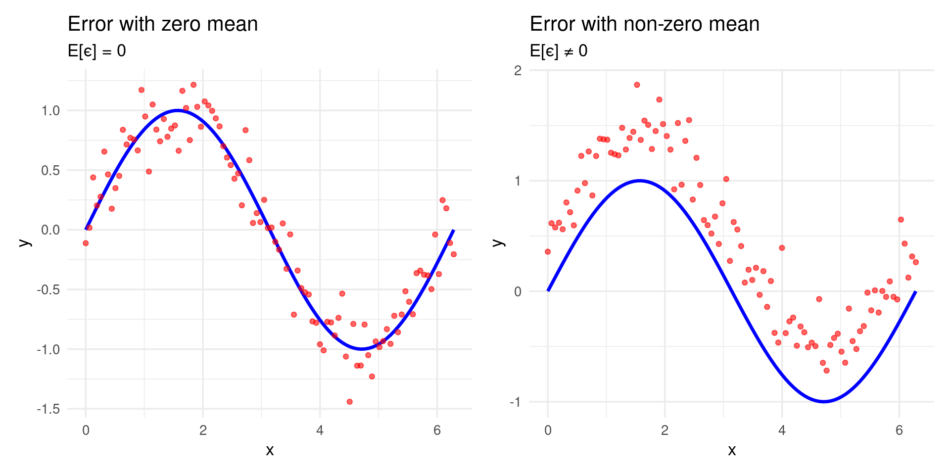
Why is the expected value of the error zero, \(E(\epsilon) = 0\)?
which implies that the noise does not affect the expected value of \(y\) given \(\dot{\mathbf{x}}\), thereby preserving the model’s unbiasedness.
Implications
\(E[\epsilon] = 0\) signifies that the noise is unbiased.
If \(E[\epsilon] \ne 0\), the model would exhibit a systematic bias.
The model would capture an incorrect mean of \(y\), negatively impacting its predictive performance.
The Two Cultures
Prediction
Example 1:
True value: \(f(x) = 170\)
Noise: \(\epsilon \sim \mathcal{N}(0, 35)\)
Model:
\[
y = 170 + \epsilon
\]
Then:
\[
E[y] = 170 + E[\epsilon] = 170 + 0 = 170
\]
The observed mean value coincides with the true value.
The Two Cultures
Prediction
Example 2: Biased Noise
True value: \(f(x) = 170\)
Noise: \(\epsilon \sim \mathcal{N}(10, 35)\)
Model:
\[
y = 170 + \epsilon
\]
Then:
\[
E[y] = 170 + E[\epsilon] = 170 + 10 = 180
\]
In this case, the observed mean is shifted. The model exhibits systematic bias.
The Two Cultures
Prediction
library(ggplot2)library(patchwork)set.seed(123)n <-100x <-seq(0, 2*pi, length.out = n)g_x <-sin(x)# Case 1: Error with zero mean (no bias)eps_zero <-rnorm(n, mean =0, sd =0.2)y_zero <- g_x + eps_zerodf_zero <-data.frame(x = x, g_x = g_x, y = y_zero)p1 <-ggplot(df_zero, aes(x = x)) +geom_line(aes(y = g_x), color ="blue", size =1.2) +geom_point(aes(y = y), alpha =0.6, color ="red") +labs(title ="Error with zero mean",subtitle ="E[ϵ] = 0",x ="x", y ="y") +theme_minimal(base_size =13)# Case 2: Error with non-zero mean (biased)eps_bias <-rnorm(n, mean =0.5, sd =0.2)y_bias <- g_x + eps_biasdf_bias <-data.frame(x = x, g_x = g_x, y = y_bias)p2 <-ggplot(df_bias, aes(x = x)) +geom_line(aes(y = g_x), color ="blue", size =1.2) +geom_point(aes(y = y), alpha =0.6, color ="red") +labs(title ="Error with non-zero mean",subtitle ="E[ϵ] ≠ 0",x ="x", y ="y") +theme_minimal(base_size =13)# Mostrar lado a ladop1 + p2
The Two Cultures
Prediction
The Two Cultures
Prediction
Example:
Consider a firm interested in conducting a direct marketing campaign.
The objective is to identify individuals likely to respond positively to a direct mailing, based on observed demographic variables measured at the individual level.
In this context, the demographic variables serve as predictors, while the marketing campaign response (binary: positive or negative) serves as the outcome variable.
The firm is not primarily concerned with attaining a profound understanding of the underlying relationships between individual predictors and the response. Instead, the focus is solely on developing an accurate model to predict response based on these predictors. This exemplifies a modeling approach centered on prediction.
How Do We Estimate \(f\)?
We shall consistently assume that we observe a set of \(n\) distinct data points. For instance, \(n = 30\) indicates a sample size of 30 observations. Based on these observations, we estimate a model \(\hat{f}\) that best approximates \(f\).
Let \(x_{ij}\) denote the value of the \(j\)-th variable for the \(i\)-th observation, where \(i = 1, 2, \ldots, n\) and \(j = 1, 2, \ldots, p\). Additionally, let \(y_i\) represent the observed value of the response variable for the \(i\)-th observation. Consequently, our dataset consists of:
where \(\dot{\mathbf{x}}_i = (x_{i1}, x_{i2}, \ldots, x_{ip})^\top\).
How Do We Estimate \(f\)?
Our objective is to apply a statistical learning method to the data in order to estimate the unknown function \(f\).
In other words, we seek to find a function \(\hat{f}\) such that \(y \approx \hat{f}(\dot{\mathbf{x}})\) for any given observation \((\dot{\mathbf{x}}, y)\).
Broadly speaking, most statistical learning methods for this task can be characterized as either parametric or non-parametric.
How Do We Estimate \(f\)?
Consider the following example:
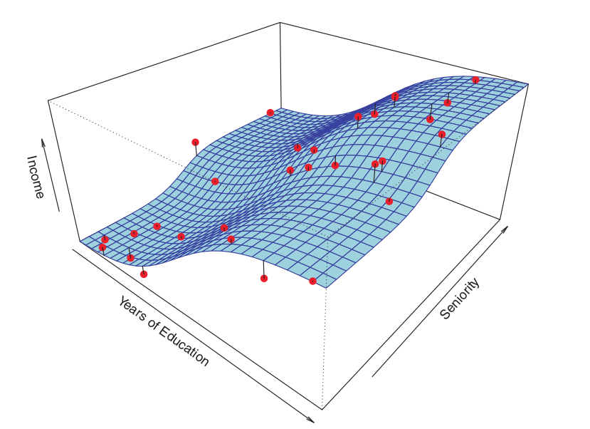
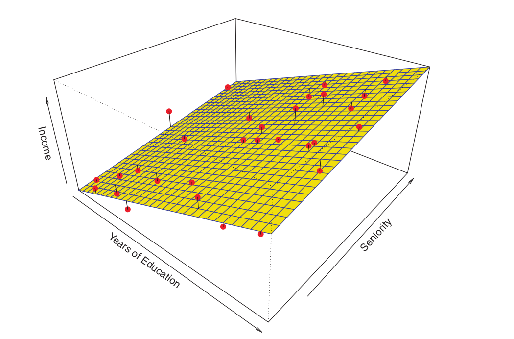
The plot illustrates income as a function of years of education and seniority within the Income dataset.
The blue surface represents the true underlying relationship between income, years of education, and seniority, which is known. The red points indicate the observed values of these variables for 30 individuals.
How Do We Estimate \(f\)?
Parametric Methods
Parametric methods involve a two-step model-based approach:
First, we make an assumption about the functional form, or shape, of \(f\). For example, a common and simple assumption is that \(f\) is linear in \(\mathbf{x}\)1:
Once we assume that \(f\) is linear, the problem of estimating \(f\) reduces to estimating the \(p + 1\) coefficients \(\beta_0, \beta_1, \ldots, \beta_p\) of the model.
How Do We Estimate \(f\)?
Parametric Methods
Once a model has been selected, we require a procedure that utilizes the data to fit or estimate the model. In the case of the linear model, we need to estimate the parameters \(\beta_0, \beta_1, \ldots, \beta_p\). We seek to find values for these parameters such that:
A well-established and widely utilized approach is (Ordinary) Least Squares.
How Do We Estimate \(f\)?
Parametric Methods
OLS - Ordinary Least Squares
Given the observations \((x_{i1}, x_{i2}, \dots, x_{ip}, y_i)\) for \(i = 1, 2, \dots, n\), we define the model: \[
y_i = \beta_0 + \beta_1 x_{i1} + \beta_2 x_{i2} + \dots + \beta_p x_{ip} + \epsilon_i
\]
where \(\epsilon_i\) is the random error term, with \(E[\epsilon_i] = 0\).
Our objective is to estimate \(\hat{\beta}_0, \hat{\beta}_1, \dots, \hat{\beta}_p\) by minimizing the errors. In this approach, we minimize the residual sum of squares (RSS): \[
S(\boldsymbol{\beta}) = \sum_{i=1}^n \left( y_i - (\hat{\beta}_0 + \hat{\beta}_1 x_{i1} + \dots + \hat{\beta}_p x_{ip}) \right)^2 = \sum_{i=1}^n (y_i - \hat{y}_i)^2 = \sum_{i=1}^n e_i^2
\]
where \(\boldsymbol{\beta} = [\beta_0 \, \beta_1\, \ldots\, \beta_p]^\top\) and \(e_i = y_i - \hat{y}_i\) represents the residual for the \(i\)-th observation, with \(\hat{y}_i\) denoting the predicted value.
How Do We Estimate \(f\)?
Parametric Methods
OLS - Ordinary Least Squares
The solution involves finding the values of \(\hat{\boldsymbol{\beta}} = [\hat{\beta_0} \, \hat{\beta_1}\, \ldots\, \hat{\beta_p}]^\top\) that minimize the objective function \(S\). This is achieved by calculating the partial derivatives of \(S(\cdot)\) with respect to each \(\beta_j\) and setting them to zero: \[
\frac{\partial S}{\partial \beta_j} = 0, \quad j = 0, 1, \dots, p
\]
Solving the resulting system of equations (the normal equations): \[
\dot{\mathbf{X}}^\top \dot{\mathbf{X}} \hat{\boldsymbol{\beta}} = \dot{\mathbf{X}}^\top \mathbf{y}
\]
\(\dot{\mathbf{X}}\): Referred to as the design matrix, observed data matrix, input matrix, or independent variable matrix, with dimensions \((n \times (p+1))\); \(\mathbf{y}\) is the response variable vector with dimensions \((n \times 1)\); \(\hat{\boldsymbol{\beta}}\) is the vector of estimated parameters with dimensions \(((p+1) \times 1)\).
How Do We Estimate \(f\)?
Parametric Methods
OLS - Ordinary Least Squares
In this case, the final solution is derived from the following equation:
Note: If the matrix \(\dot{\mathbf{X}}^\top \dot{\mathbf{X}}\) is non-invertible (singular), the aforementioned equation does not possess a unique solution.
How Do We Estimate \(f\)?
Parametric Methods
The approach described above is referred to as parametric, as it reduces the problem of estimating \(f\) to the estimation of a specific set of parameters.
Assuming a parametric form for \(f\) simplifies the estimation process because it is generally much easier to estimate a fixed set of parameters—such as \(\beta_0, \beta_1, \ldots, \beta_p\) in a linear model—than to fit a completely arbitrary function \(f\).
A potential drawback of a parametric approach is that the chosen model typically does not match the true, unknown functional form of \(f\).
If the selected model is highly discrepant from the true \(f\), the resulting estimate will be poor.
How Do We Estimate \(f\)?
Parametric Methods
The figure below illustrates an example of the parametric approach applied to the Income dataset1.
Since we assume a linear relationship between the response and the two predictors, the entire fitting process reduces to estimating \(\beta_0, \beta_1\), and \(\beta_2\), which is performed using ordinary least squares linear regression.
While the linear fit shown in the Figure is not perfect, it nonetheless appears to perform reasonably well in capturing the positive association between years of education and income, as well as the slightly less pronounced positive relationship between seniority and income.
How Do We Estimate \(f\)?
Non-parametric Methods
Non-parametric methods do not make explicit assumptions concerning the functional form of \(f\).
Instead, they seek an estimate of \(f\) that approximates the data points as closely as possible, without being excessively rough or oscillatory.
By avoiding the assumption of a specific functional form for \(f\), these methods have the potential to accurately fit a wider range of possible shapes for \(f\).
How Do We Estimate \(f\)?
Non-parametric Methods
Any parametric approach carries the risk that the functional form used to estimate \(f\) may deviate significantly from the true \(f\), in which case the resulting model will yield a poor fit to the data. In contrast, non-parametric approaches circumvent this danger entirely, as they essentially make no prior assumptions regarding the functional form of \(f\).
However, non-parametric approaches suffer from a major drawback: since they do not reduce the problem of estimating \(f\) to a small number of parameters, a much larger number of observations (considerably higher than what is typically required for a parametric approach) is necessary to obtain an accurate estimate of \(f\).
How Do We Estimate \(f\)?
Non-parametric Methods
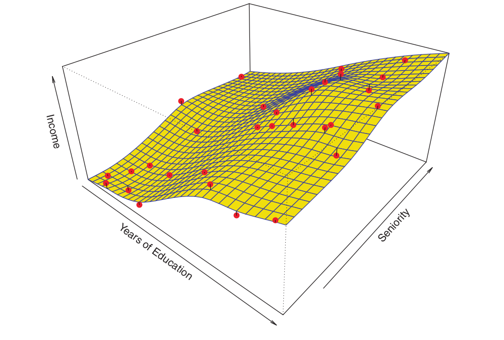
An example of a non-parametric approach for fitting the Income dataset is illustrated in the figure below1.
How Do We Estimate \(f\)?
Non-parametric Methods
A thin-plate spline1 was utilized to estimate \(f\).
This approach does not impose any pre-specified model on \(f\). Instead, it attempts to produce an estimate for \(f\) that is as close as possible to the observed data, subject to the constraint that the fit (the yellow surface in the Figure) remains smooth.
In this instance, the non-parametric fit yielded an insightful estimate for \(f\).
How Do We Estimate \(f\)?
Non-parametric Methods
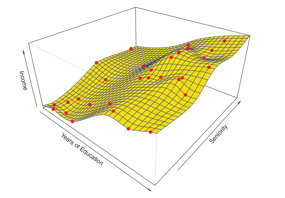
The figure below illustrates the same thin-plate spline fit employing a lower level of smoothness1, allowing for a more irregular fit.
How Do We Estimate \(f\)?
Non-parametric Methods
The resulting estimate yields a near-perfect fit to the observed data points.
This serves as a quintessential example of overfitting.
This is an undesirable situation because the resulting fit fails to provide accurate response estimates for unseen observations that were not part of the original training dataset.
How Do We Estimate \(f\)?
Parametric and Non-parametric Methods
Trade-Off Between Prediction and Inference
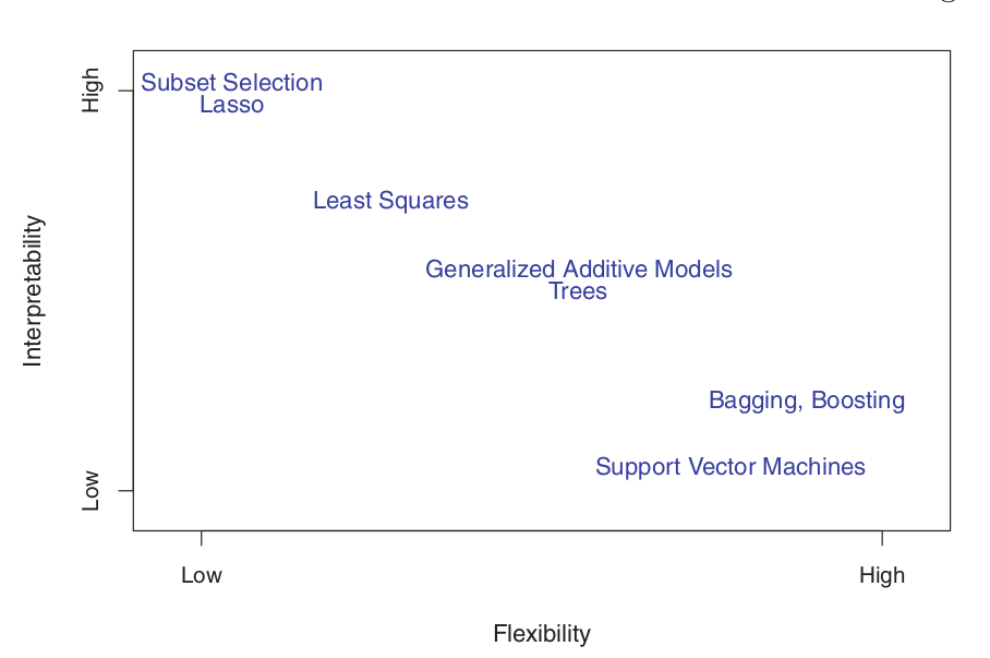
The Balance Between Prediction Accuracy and Model Interpretability
Why would we choose to employ a more restrictive (parametric) method instead of a more flexible (non-parametric) approach?
If the primary interest lies in inference, more restrictive models are inherently more interpretable.
For instance, when inference is the goal, parametric models are often preferred choices, as they allow for a clear understanding of the functional relationship between \(Y\) and \(X_1, X_2, \ldots, X_p\).
Trade-Off Between Prediction and Inference
Ordinary Least Squares (OLS) linear regression is relatively inflexible but highly interpretable.
Lasso regression is based on the linear model but employs an alternative procedure to estimate the coefficients \(\beta_0, \beta_1, \ldots, \beta_p\). This procedure is more restrictive during estimation and shrinks some coefficients to exactly zero. Consequently, in this sense, Lasso is a less flexible approach than ordinary linear regression. It is also more interpretable than linear regression because, in the final model, the response variable is associated with only a small subset of the predictors—specifically those with non-zero coefficient estimates.
Trade-Off Between Prediction and Inference
Generalized Additive Models (GAMs) extend the linear model to accommodate specific non-linear relationships. Consequently, GAMs are more flexible and slightly less interpretable compared to linear regression.
Fully non-linear methods, such as bagging, boosting, and Support Vector Machines (SVM) with non-linear kernels, are highly flexible approaches that are significantly more challenging to interpret.
Trade-Off Between Prediction and Inference
Based on the preceding discussion, we have established that when inference is the primary objective, there are distinct advantages to employing relatively inflexible statistical learning methods.
In certain scenarios, however, we are solely interested in prediction, and the interpretability of the predictive model is essentially irrelevant.
In such a case, one might expect that the optimal strategy would be to utilize the most flexible model available.
Frequently, however, we obtain more accurate predictions by using a less flexible method.
This phenomenon, which may seem counter-intuitive at first glance, is related to the potential for overfitting in highly flexible methods.
An Introduction to Statistical Learning: with Applications in R, James, G., Witten, D., Hastie, T. and Tibshirani, R., Springer, 2013, link: https://www.statlearning.com/.
Mathematics for Machine Learning, Deisenroth, M. P., Faisal. A. F., Ong, C. S., Cambridge University Press, 2020, link: https://mml-book.com.
References
Complementary
An Introduction to Statistical Learning: with Applications in python, James, G., Witten, D., Hastie, T. and Tibshirani, R., Taylor, J., Springer, 2023, link: https://www.statlearning.com/.
Matrix Calculus (for Machine Learning and Beyond), Paige Bright, Alan Edelman, Steven G. Johnson, 2025, link: https://arxiv.org/abs/2501.14787.