\(\boldsymbol{\theta}\) denotes the model parameters;
\(\dot{\mathbf{x}}\) is an input vector;
\(\theta_0\) is a bias term;
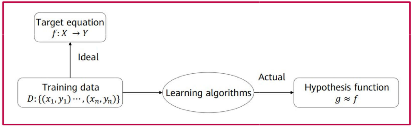
Models as Functions
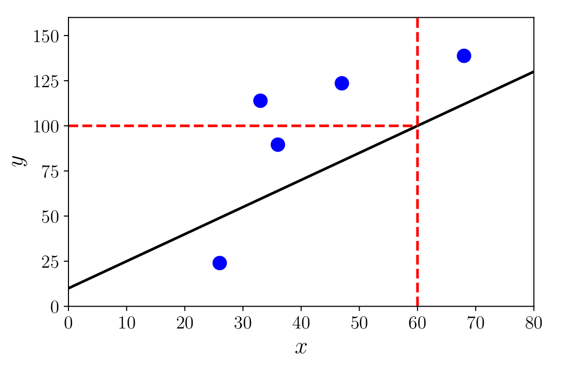
Example: Linear Regression
Function (solid black diagonal line) and its prediction at \(x = 60\), i.e., \(f(60) = 100\).
Probabilistic Models
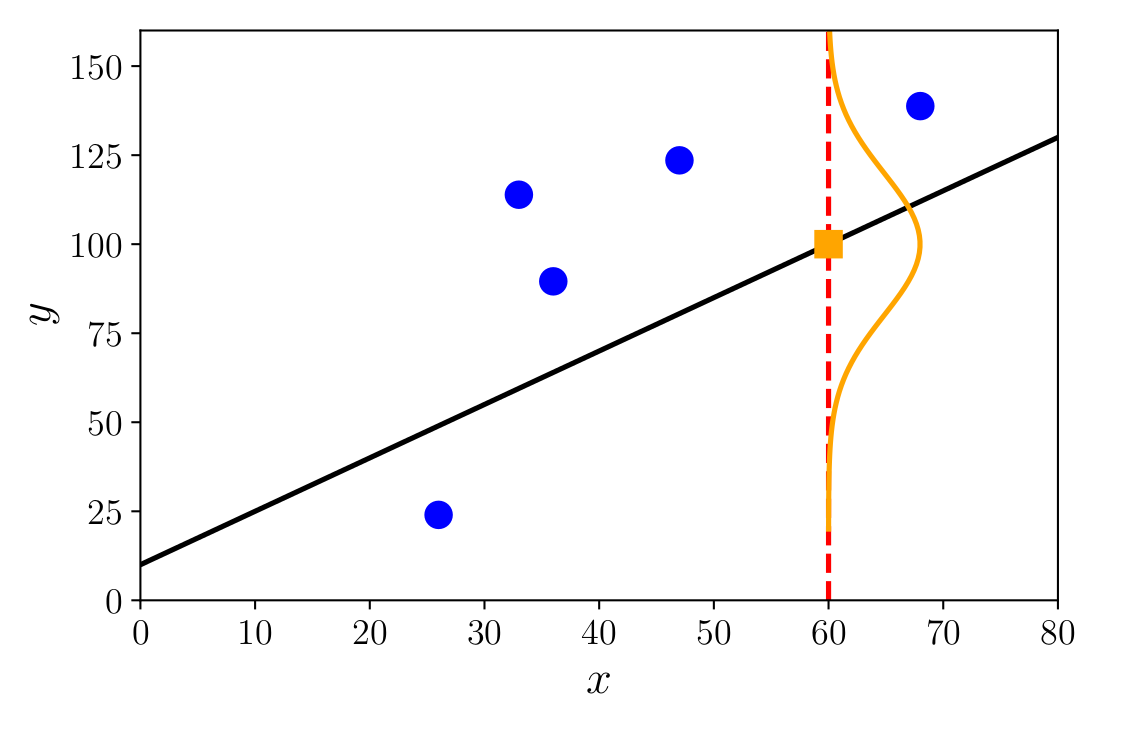
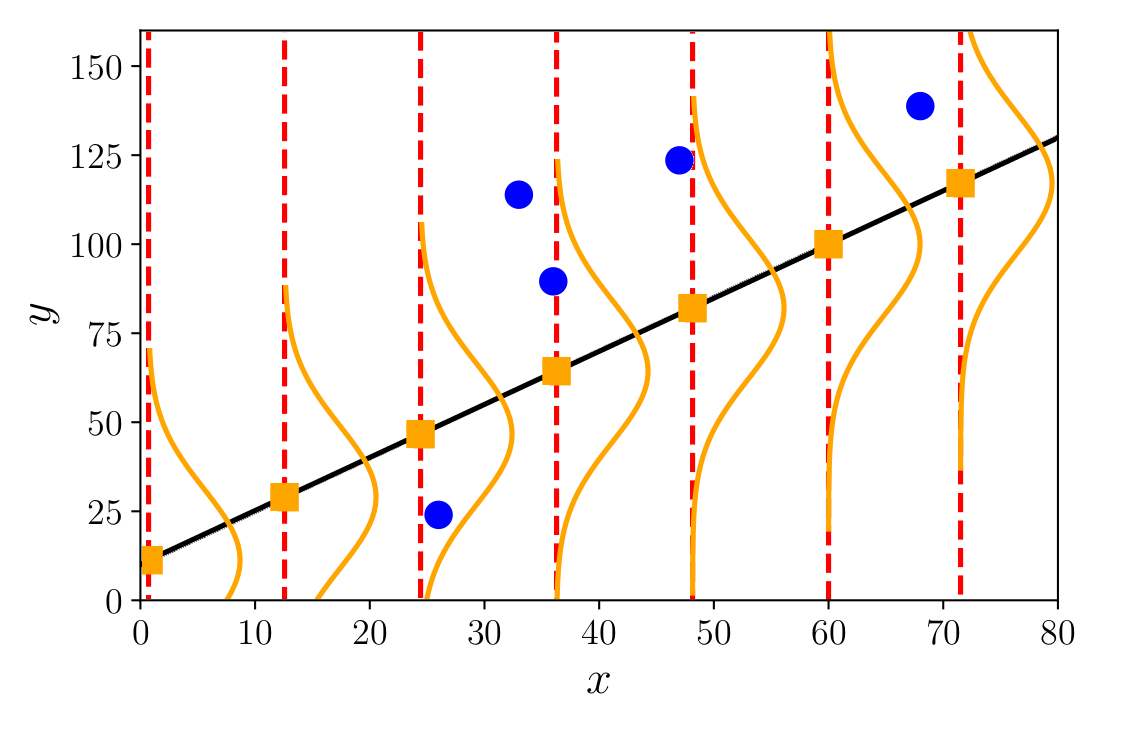
In probabilistic models, we associate a probability distribution with the data, thereby incorporating uncertainty through these distributions.
In the example below, featuring regression with Gaussian noise, it is assumed that the value \(y_i\) follows a normal distribution centered at \(\boldsymbol{\theta}^\top \dot{\mathbf{x}}_i\):
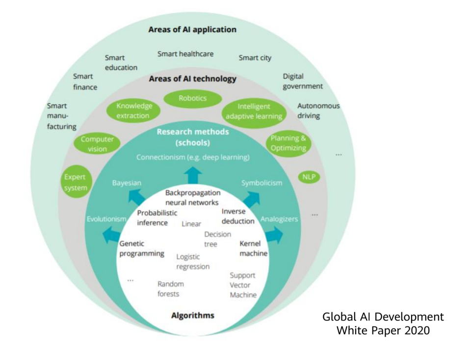
Supervised Learning – algorithms trained on labeled data to map inputs to target outputs.
Unsupervised Learning – algorithms that perform clustering and derive inferences from unlabeled datasets.
Reinforcement Learning – algorithms that learn through trial and error by interacting with a dynamic environment.
Machine Learning
Key concepts include:
Supervised Learning – algorithms trained on labeled data to map inputs to target outputs.
Unsupervised Learning – algorithms that cluster and derive inferences from unlabeled datasets.
Reinforcement Learning – algorithms that learn through trial and error by interacting with a dynamic environment.
Supervised Learning - ML
Supervised Learning
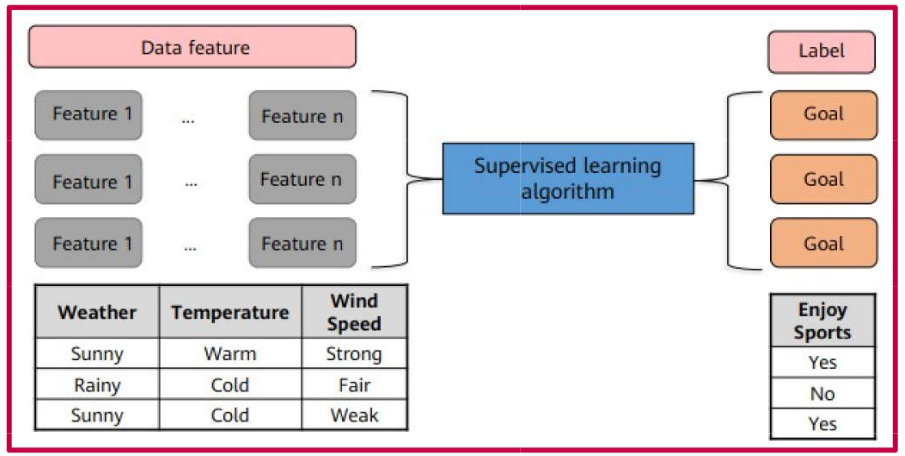
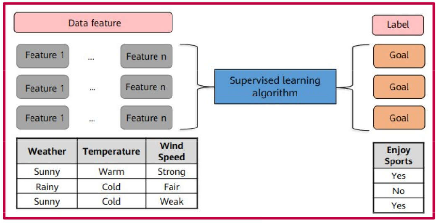
Supervised learning is the most prevalent form of machine learning. It is employed to predict an outcome based on a set of input variables.
It is termed “supervised” because the algorithm learns from a labeled dataset—that is, a dataset containing both inputs and their corresponding desired outputs.
Supervised learning is utilized across a wide range of applications, typically involving classification and regression algorithms.
Supervised Learning - ML
When the target output is a qualitative variable \((y \in \mathbb{N})\), the task is referred to as CLASSIFICATION.
An optimized model is obtained through training and learning based on observations \(\mathbf{x}_i\), for \(i = 1, 2, \ldots, n\), for which the corresponding desired response \(y_i\) is available.
Each observation \(\mathbf{x}_i\) may consist of \(p\) independent variables (features)\(\mathbf{x}_i = x_{i1}, x_{i2}, \ldots, x_{ip}\), where \(p \geq 1\).
Supervised Learning - ML
The objective is to utilize the developed model to map new inputs.
When the desired output is a quantitative variable—belonging either to the set of integers \((y \in \mathbb{Z})\) or real numbers \((y \in \mathbb{R})\)1, the task is referred to as REGRESSION2.
Examples:
What is the average weight of soccer players?
What was the average temperature in Recife over the last month?
What is the market value of a \(100m^2\) apartment in Boa Viagem?
Unsupervised Learning - ML
Unsupervised Learning
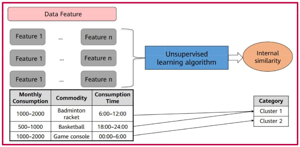
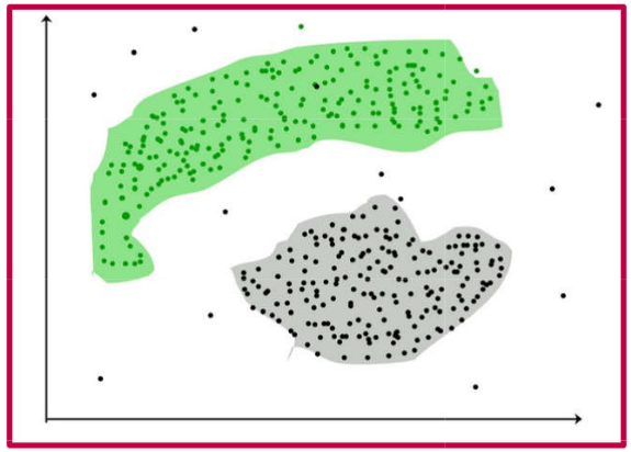
Unsupervised learning is the branch of machine learning employed to derive inferences from unlabeled datasets.
It is termed “unsupervised” because the algorithm is not trained on labeled data. Instead, the algorithm identifies underlying patterns within the training data and is capable of making inferences about new data.
Unsupervised learning is utilized across a wide range of applications, primarily through clustering and dimensionality reduction algorithms.
Unsupervised Learning - ML
An optimized model is obtained by directly processing input data without prior knowledge of the target output. As before, we have a set of observations \(\mathbf{x}_i\), where \(i = 1, 2, \ldots, n\) and \(p \geq 1\) features.
Unsupervised Learning - ML
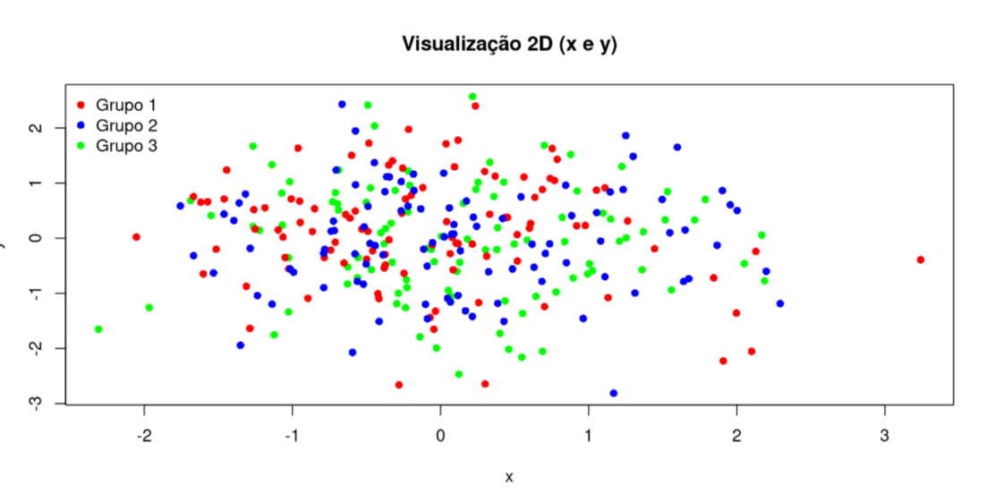
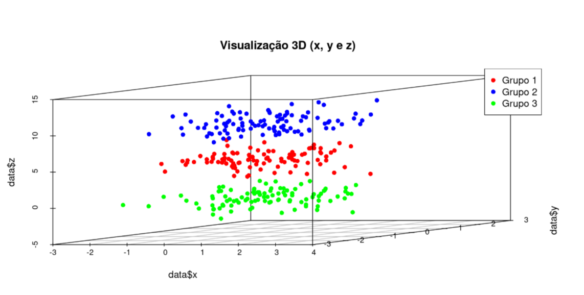
Clustering is the most prevalent unsupervised learning technique. It is used to partition data into groups (clusters) based on their characteristics (variables, features).
While typically applied to a dataset where the identified clusters represent the primary objective, it is also possible to assign new observations to these established groups based on the similarity between the new data points and the existing cluster members.
Unsupervised Learning - ML
Unsupervised Learning - ML
Unsupervised Learning - ML
Reinforcement Learning - ML
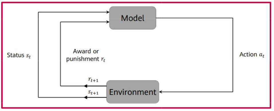
Instead of a static sample, the process involves a sequence of actions performed within an environment; the algorithm learns the optimal policy to maximize a cumulative reward.
For every action, feedback is provided, indicating whether the action was favorable or unfavorable.
For example: Winning a game of checkers (draughts) after a series of strategic moves.
Reinforcement Learning - ML
The objective is for the algorithm to control the robotic arm and learn how to reach the red target.
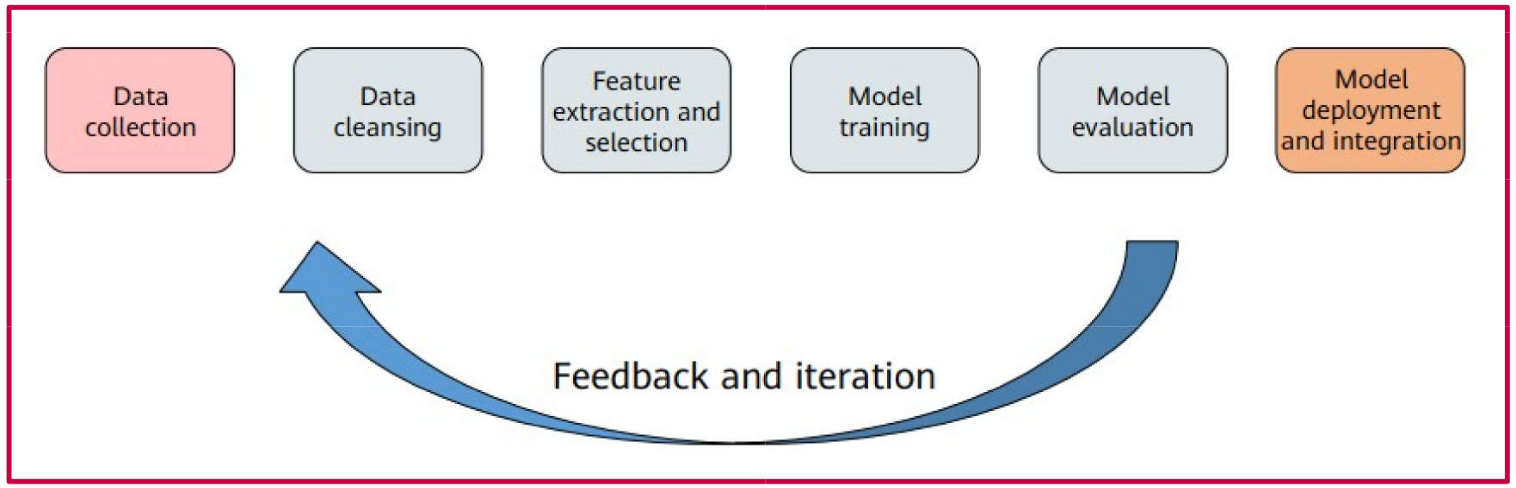
ML: The Learning Process
Figure 1
Note that the process is iterative, meaning that revisiting previous stages is necessary to refine the model.
ML: The Learning Process
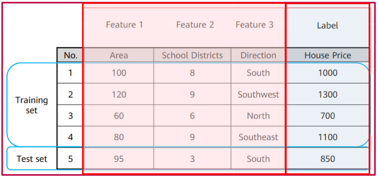
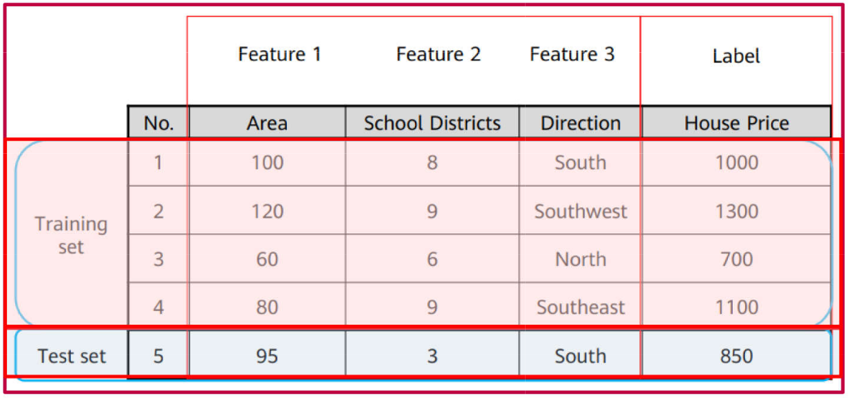
Data Organization
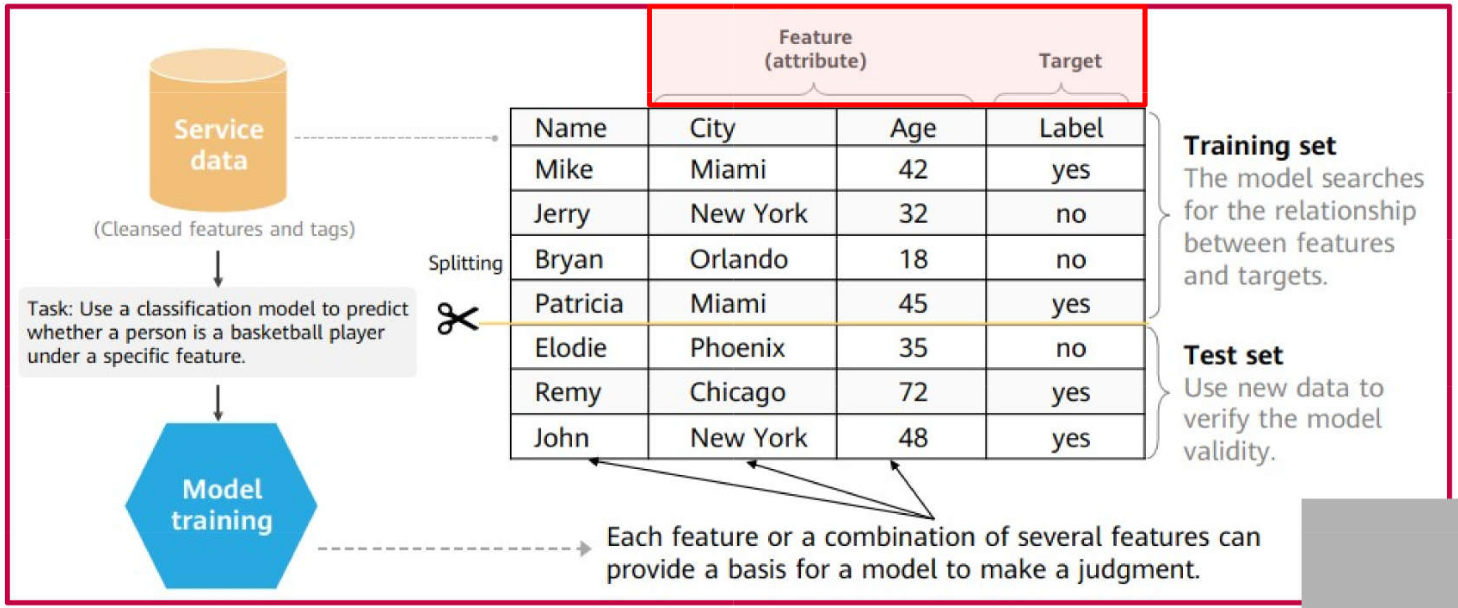
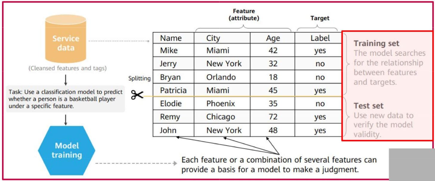
Dataset: Broadly refers to the collection of data utilized in machine learning. Each record is termed an observation, example, instance, or sample, and is composed of variables or features. Features represent the relevant attributes used to characterize the observations.
Training Set: The data subset used to train the model (learning phase). It comprises a set of observations along with their corresponding target outputs.
Test Set: The data subset used to evaluate the trained model. It simulates real-world scenarios where the model is applied to unseen data. It consists of a set of input observations.
ML: The Learning Process
Example of a Labeled Dataset:
ML: The Learning Process
Example of a Labeled Dataset:
ML: The Learning Process
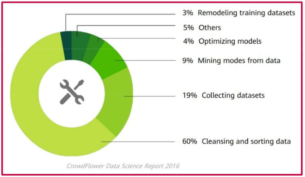
Importance of Data
If the data is good, there is no guarantee that the model will be good
If the data is not good, we can guarantee that the model will be bad
Preprocessing Steps
Cleaning\(\rightarrow\) Removal of duplicate data, outliers, missing data, avoiding inconsistencies and errors in data reading;
Dimensionality Reduction\(\rightarrow\) Avoiding dimensionality explosion by reducing the number of variables;
Normalization\(\rightarrow\) Standardizing the data, preventing variables with different scales from influencing the model, reducing noise, and improving model performance;
ML: The Learning Process
The process begins with data cleaning, but note the division of work using real data, raw data, and clean data, which is the result of the cleaning process.
ML: The Learning Process
Data Cleaning
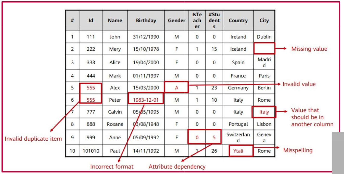
Generally, machine learning models do not perform well with missing, duplicate, or inconsistent data.
It is common to have collected data that can only be used after a preparation step, which may include:
Removal of duplicate data;
Handling of missing data;
Handling of outliers;
Data normalization;
Dimensionality reduction;
Transformation of categorical variables into numerical ones;
Class balancing (e.g., in classification problems with imbalanced classes);
ML: The Learning Process
Examples of issues encountered in raw data:
ML: The Learning Process
Data Conversion
The conversion stage occurs between preprocessing and feature selection; it entails transforming the data into a format suitable for the model.
Examples include:
Conversion of categorical variables into numerical values;
Conversion of numerical variables into categorical ones (discretization);
Conversion of temporal variables into numerical representations;
Conversion of textual data into numerical vectors (e.g., word embeddings, Word2Vec, BERT);
Conversion of images into numerical representations (tensors/arrays);
Conversion of audio signals into numerical formats.
ML: The Learning Process
Data Conversion
Image data can be transformed using:
Color space mapping;
Grayscale conversion;
Color histograms;
Feature Engineering: The process of creating new variables from the original feature set.
Feature normalization: Adjusting features to standardize their value ranges;
Feature expansion: Combining or transforming variables to generate novel features;
ML: The Learning Process
Post-cleaning and conversion…
Feature Selection \(\rightarrow\) Motivations
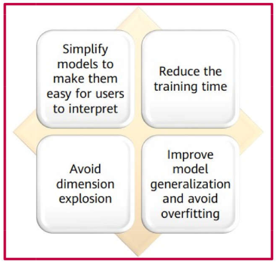
Datasets typically contain a high dimensionality of features. Some may be redundant or irrelevant to the target prediction and, therefore, can be excluded.
This stage is independent of the specific machine learning algorithm employed (algorithm-agnostic).
There are four primary motivations for implementing feature selection.
ML: The Learning Process
Feature Selection \(\rightarrow\) Methods
Three main categories of methods are highlighted:
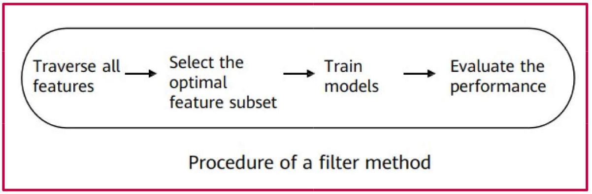
Filter methods: Techniques that select features based on statistical metrics, such as correlation, entropy, and others.
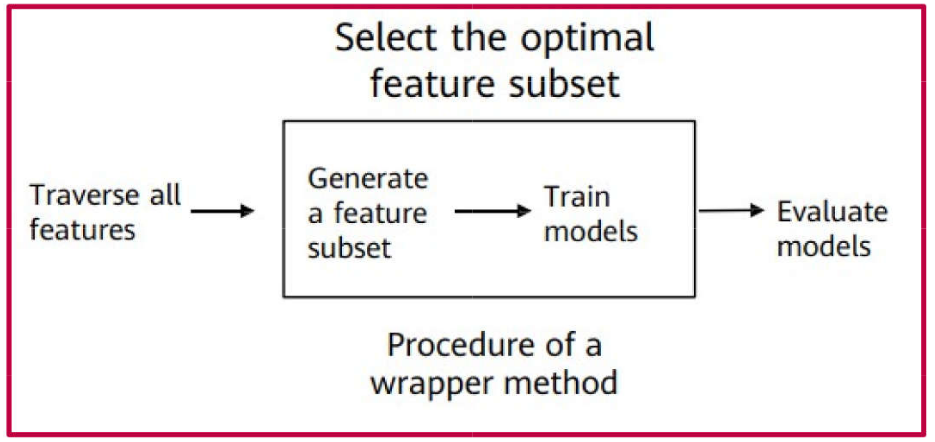
Wrapper methods: Techniques that select features based on the predictive performance of a specific machine learning model.
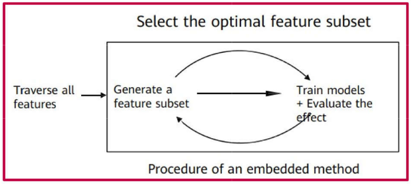
Embedded methods: Techniques that perform feature selection natively during the model training process.
ML: The Learning Process
Feature Selection \(\rightarrow\) Filter Methods
This category encompasses techniques based on the correlation between features and the target variable.
Generally, these methods utilize statistical parameters to select the most relevant features by applying a threshold or establishing a feature ranking.
ML: The Learning Process
Feature Selection \(\rightarrow\) Filter Methods
Common Methods:
Pearson Correlation: measures the linear relationship between two continuous variables.
Spearman Correlation: assesses the monotonic relationship between continuous or ordinal variables.
Kendall Correlation: evaluates the ordinal association between two ordinal variables.
Chi-Square Test: measures the dependency between two categorical variables.
Limitations:
Does not account for dependencies or interactions between features;
Fails to capture non-linear relationships between features and the target variable;
Typically evaluates features in isolation rather than considering their combined predictive power.
ML: The Learning Process
Feature Selection \(\rightarrow\) Wrapper Methods
This category encompasses techniques that utilize a machine learning model to evaluate feature importance.
Generally, these methods employ a machine learning algorithm to assess the significance of features and select the most relevant subset.
ML: The Learning Process
Feature Selection \(\rightarrow\) Wrapper Methods
Common Methods:
Forward Selection: Begins with a null model and adds features one at a time, evaluating the model’s performance at each iteration.
Backward Elimination: Starts with a full model containing all features and removes them sequentially, assessing the model’s performance at each step.
Stepwise Selection: A bidirectional approach that combines both forward and backward selection techniques.
Recursive Feature Elimination (RFE): Iteratively removes features based on the importance weights assigned by the model.
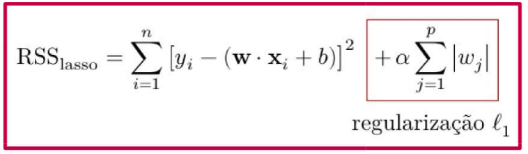
Lasso (Least Absolute Shrinkage and Selection Operator): Incorporates an L1 regularization penalty into the cost function, effectively performing feature selection by shrinking some coefficients to zero.
Ridge: Adds an L2 regularization penalty to the cost function to prevent multicollinearity and control model complexity.
Random Forest, XGBoost, LightGBM, CatBoost: These algorithms evaluate feature importance based on impurity reduction (e.g., Gini impurity or entropy); thus, feature significance is assessed natively during the model training process.
Often referred to as L1 penalty methods, they incorporate an L1 regularization term into the cost function. This method imposes constraints during the model optimization process, shrinking the coefficients of certain features to exactly zero, thereby effectively eliminating them from the model.
For example: weights of redundant features are naturally nullified…
ML: The Learning Process
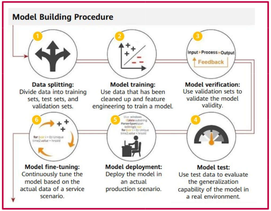
General overview of the model construction process (Steps 1 through 6). Note the significance of Step 2!
ML: The Learning Process
An example of Supervised Learning \(\rightarrow\) The Learning Phase
ML: The Learning Process
An example of Supervised Learning \(\rightarrow\) The Learning Phase
ML: The Learning Process
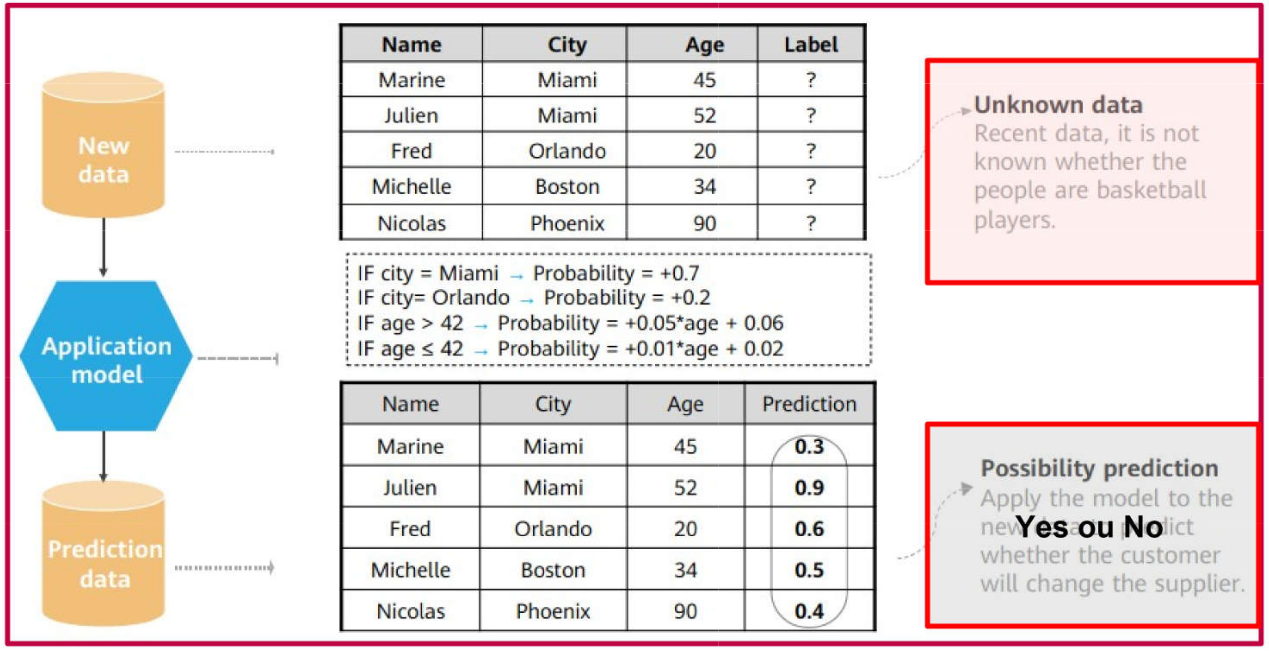
An example of Supervised Learning \(\rightarrow\) The Prediction Phase
ML: The Learning Process
What defines a “good” model?
What are the right questions to ask?
Accuracy: Does the model predict correctly? i.e., is the model’s predictive performance high?
Interpretability: Is the model comprehensible? i.e., is it possible to understand the logic behind a specific prediction?
Robustness: Is the model resilient to noise? i.e., can it maintain performance despite perturbations in the data?
Scalability: Is the model scalable? i.e., is it capable of processing large-scale datasets efficiently?
Generalization: Does the model generalize well? i.e., is it capable of providing accurate predictions for unseen data?
Efficiency: Is the model computationally efficient? i.e., can it generate predictions within a reasonable timeframe (low latency)?
ML: The Learning Process
Model Validity - Definitions
Generalization Capability: The ability of the model to provide accurate predictions for unseen data.
Error: The discrepancy between the predicted value and the ground truth (actual value). There are two primary types:
Training Error: The error calculated between the predicted and actual values within the training set.
Test Error: The error calculated between the predicted and actual values within the test set.
Model Capacity: The model’s ability to fit the training data effectively while maintaining its ability to generalize to new data.
Conclusions
The Learning Process
Preprocessing: Feature encoding and Normalization (where applicable)
Training: Conducted via optimization methods
Evaluation: Performed through performance metrics and cross-validation
Ethics in Machine Learning
Privacy: Data anonymization and de-identification (e.g., removing personal identifiers)
Bias: Critical assessment of features and algorithmic outcomes
Transparency: Model interpretability and explainability
An Introduction to Statistical Learning: with Applications in R, James, G., Witten, D., Hastie, T. and Tibshirani, R., Springer, 2013, link: https://www.statlearning.com/.
Mathematics for Machine Learning, Deisenroth, M. P., Faisal. A. F., Ong, C. S., Cambridge University Press, 2020, link: https://mml-book.com.
References
Complementary
An Introduction to Statistical Learning: with Applications in python, James, G., Witten, D., Hastie, T. and Tibshirani, R., Taylor, J., Springer, 2023, link: https://www.statlearning.com/.
Matrix Calculus (for Machine Learning and Beyond), Paige Bright, Alan Edelman, Steven G. Johnson, 2025, link: https://arxiv.org/abs/2501.14787.