Statistical Machine Learning
Introduction to Python
UFPE
Virtual Environments
In Python, we generally use virtual environments to isolate project dependencies. This is useful so that we can have different versions of the same library in different projects.
Anaconda is a virtual environment manager and has been the most widely used in recent years by data scientists, developers, and data engineers who use Python. The advantage of using Anaconda is that it comes pre-installed with several libraries, which facilitates the data scientist’s workflow.
To download Anaconda, visit the link: https://www.anaconda.com/products/distribution and download the latest version for your operating system.
Anaconda
Several commands are essential for using Anaconda, such as:
- Creating a virtual environment:
conda create -n environment_name python=3.11.5 - Listing virtual environments:
conda env list - Activating a virtual environment:
conda activate environment_name - Deactivating a virtual environment:
conda deactivate - Removing a virtual environment:
conda env remove -n environment_name
Anaconda
- Library installations are performed using the
conda install library_namecommand, but Python libraries are generally installed using pip, which is the Python package manager. To install a library using pip, we use the commandpip install library_name.
For example, to install the pandas library, we use the command:
And we can verify if the installation was successful using:
Name: pandas
Version: 2.1.4
Summary: Powerful data structures for data analysis, time series, and statistics
Home-page: https://pandas.pydata.org
Author:
Author-email: The Pandas Development Team <pandas-dev@python.org>
License: BSD 3-Clause License

Copyright (c) 2008-2011, AQR Capital Management, LLC, Lambda Foundry, Inc. and PyData Development Team
All rights reserved.

Copyright (c) 2011-2023, Open source contributors.

Redistribution and use in source and binary forms, with or without
modification, are permitted provided that the following conditions are met:

* Redistributions of source code must retain the above copyright notice, this
  list of conditions and the following disclaimer.

* Redistributions in binary form must reproduce the above copyright notice,
  this list of conditions and the following disclaimer in the documentation
  and/or other materials provided with the distribution.

* Neither the name of the copyright holder nor the names of its
  contributors may be used to endorse or promote products derived from
  this software without specific prior written permission.

THIS SOFTWARE IS PROVIDED BY THE COPYRIGHT HOLDERS AND CONTRIBUTORS "AS IS"
AND ANY EXPRESS OR IMPLIED WARRANTIES, INCLUDING, BUT NOT LIMITED TO, THE
IMPLIED WARRANTIES OF MERCHANTABILITY AND FITNESS FOR A PARTICULAR PURPOSE ARE
DISCLAIMED. IN NO EVENT SHALL THE COPYRIGHT HOLDER OR CONTRIBUTORS BE LIABLE
FOR ANY DIRECT, INDIRECT, INCIDENTAL, SPECIAL, EXEMPLARY, OR CONSEQUENTIAL
DAMAGES (INCLUDING, BUT NOT LIMITED TO, PROCUREMENT OF SUBSTITUTE GOODS OR
SERVICES; LOSS OF USE, DATA, OR PROFITS; OR BUSINESS INTERRUPTION) HOWEVER
CAUSED AND ON ANY THEORY OF LIABILITY, WHETHER IN CONTRACT, STRICT LIABILITY,
OR TORT (INCLUDING NEGLIGENCE OR OTHERWISE) ARISING IN ANY WAY OUT OF THE USE
OF THIS SOFTWARE, EVEN IF ADVISED OF THE POSSIBILITY OF SUCH DAMAGE.
Location: /home/jodavid/anaconda3/lib/python3.11/site-packages
Requires: numpy, python-dateutil, pytz, tzdata
Required-by: altair, category-encoders, datasets, datashader, gradio, holoviews, hvplot, mizani, panel, plotly-resampler, plotnine, pmdarima, pycaret, pymilvus, satveg-api, seaborn, sktime, statsmodels, streamlit, sweetviz, TTS, xarray
Note: you may need to restart the kernel to use updated packages.
Modules
Also known as libraries, modules are files containing functions, variables, and classes that can be used in other programs.
To use a module in Python, we use the command
import module_name. If you want to use only a specific function from a module, we use the commandfrom module_name import function_name.For example, using the
mathmodule:
Above, math is the module and sqrt is the function that calculates the square root of a number.
Modules
- In Python, it is common to use module abbreviations to facilitate the use of their functions. For example, the
pandasmodule is commonly abbreviated aspd, thenumpymodule asnp, thematplotlibmodule asplt, among others.
It is worth noting that these abbreviations are embraced by the community; that is, it is not a strict rule, but it is a best practice to, for example, abbreviate pandas as pd, numpy as np, matplotlib as plt, and this applies to many other libraries.
Modules
There is also the case where you explicitly specify the functions you want from modules to use the function name directly, without the need to call the module. For example, instead of using math.sqrt(25), you can use from math import sqrt and then use sqrt(25).
Note that the
sqrtfunction was imported directly from themathmodule, and therefore it is not necessary to call the module to use it. In other words, if the function is not used as shown above and you useimport math, it is necessary to usemath.sqrt(25)to get the result, specifying that thesqrtfunction belongs to themathmodule.
Modules
- Python also allows you to use an alias for the imported function. For example, instead of using
from math import sqrt, you can usefrom math import sqrt as square_root, and then usesquare_root(25)to get the result. This is useful when the imported function has a very long name, or when the imported function’s name is very common and could cause confusion with other functions. So, an example for this case is:
Loops and Conditionals

Loops and Conditionals
- Many languages use braces to delimit blocks of code, but in Python, indentation is used for this purpose. Indentation is an essential part of the Python language and is often a source of errors for programmers who are starting to learn the language.
# Conditional example
x = 10
if x > 5:
    print("x is greater than 5")
else:
    print("x is less than or equal to 5")
x is greater than 5- As seen above, the code block inside the
ifandelsestatements is indented, meaning it has extra spacing relative to the code block outside. This is necessary for Python to understand that the code block belongs to theifandelsestatements.
Loops and Conditionals
When loops use for and while, indentation is also required to delimit the code block within the loop.
An important note: unlike the
Rlanguage, Python starts its indexing at 0. This means the first element of a list, for example, is element 0, the second element is element 1, and so on. InR, indexing starts at 1.
Complex Loops
- In Python, if you have a list, it is possible to access the list elements directly from the iteration in the
forloop. This is very useful when you want to access the index and the value of a list element.
Complex Loops
- In Python, if you have a list, it is possible to access the elements of the list directly from the iteration in the
forloop. This is very useful when you want to access the index and the value of a list element.
Complex Loops
- A more complex way is using the
enumeratefunction to access both the index and the value of a list element.
# Example of a for loop accessing the index and the value
lista = [10, 20, 30, 40, 50]
for i, value in enumerate(lista):
    print(f"Element {i} of the list is {value}")
Element 0 of the list is 10
Element 1 of the list is 20
Element 2 of the list is 30
Element 3 of the list is 40
Element 4 of the list is 50- But let’s move forward step by step and see how we can create functions in Python.
Functions
In Python, functions are created using the def keyword, followed by the function name, parentheses, and a colon. The code block inside the function is indented, meaning it has an extra space relative to the code block outside the function.
To call the function, simply use the function name followed by parentheses.
Following best programming practices, it is recommended that functions have arguments and docstrings—that is, parameters passed to the function and a header within the function explaining what each argument represents, respectively. This makes the function more flexible and useful.
Functions
An example of a function with arguments and a docstring is:
In the example above, the greet function has two arguments, name and greeting, where name is required and greeting is optional because it has a default value. Additionally, the function includes a header (docstring) that explains what each argument represents.
Functions
Python also features so-called anonymous functions or lambda functions, which are functions without a name used to create simple and quick functions.
Interestingly, lambda functions can be used in conjunction with the map, filter, and reduce functions to perform operations on lists.
Functions
It is also possible to assign lambda functions to variables, as shown in the example below:
However, most people will prefer and tell you to use def instead of lambda, as def is more readable and easier to understand.
For example:
Strings
Strings can be delimited by single or double quotes and can be accessed like lists, meaning it is possible to access each character of the string using indexing.
# String example
single_quoted_string = 'data science'
double_quoted_string = "data science"
single_quoted_string == double_quoted_stringTruePython uses backslashes to encode special characters. For example, to include a single quote in a string delimited by single quotes, you must use \'.
Strings
It is also possible to create multi-line strings using triple single or double quotes.
# Multi-line string example
multi_line_string = """This is the first line.
and this is the second line
and this is the third line"""
print(multi_line_string)
This is the first line.
and this is the second line
and this is the third linePython also features a variety of functions for manipulating strings, such as the split function, which divides a string into a list of substrings.
Lists
Lists are one of the most important data structures in Python. They are similar to vectors in other languages, such as the R language1, but they are more versatile. They are more flexible because they can store any data type and are not limited to a single data type.
# List example
integer_list = [1, 2, 3]
heterogeneous_list = ["string", 0.1, True]
list_of_lists = [integer_list, heterogeneous_list, []]
list_length = len(integer_list)
list_sum = sum(integer_list)

print(integer_list)
print(heterogeneous_list)
print(list_of_lists)
print(list_length)
print(list_sum)
[1, 2, 3]
['string', 0.1, True]
[[1, 2, 3], ['string', 0.1, True], []]
3
6Lists
You can access or modify the i-th element of a list using square brackets.
Lists
Additionally, Python has a slicing syntax that allows you to access multiple elements of a list.
# List slicing example
first_three = x[:3]
three_to_end = x[3:]
one_to_four = x[1:5]
last_three = x[-3:]
without_first_and_last = x[1:-1]
copy_of_x = x[:]

print(first_three)
print(three_to_end)
print(one_to_four)
print(last_three)
print(without_first_and_last)
print(copy_of_x)
[-1, 1, 2]
[3, 4, 5, 6, 7, 8, 9]
[1, 2, 3, 4]
[7, 8, 9]
[1, 2, 3, 4, 5, 6, 7, 8]
[-1, 1, 2, 3, 4, 5, 6, 7, 8, 9]Lists
An interesting operation is using the in operator to check if an element is contained in a list.
NOTE: This operation is much slower in lists than in dictionaries and sets, because Python performs a linear search in lists—meaning it checks the elements of the list one at a time. Consequently, checking in a set or dictionary is very fast. We will study sets and dictionaries later on.
With lists, we can also concatenate, that is, add more information to the list. This can be done in several ways, such as adding elements to the list, joining multiple lists, or multiplying lists. Below are examples of how to do this.
Lists
Lists
Tuples
We have reached Tuples, and what are they? Tuples are very similar to lists, but with one fundamental difference: they are immutable. This means once you create a tuple, you cannot add, remove, or modify its elements. Tuples are generally used for functions that return multiple values. Let’s look at some examples:
Tuples
Another example:
# Tuple example
def sum_and_product(x, y):
    return (x + y), (x * y)

sp = sum_and_product(2, 3)
s, p = sum_and_product(5, 10)
print(sp)
print(s)
print(p)
(5, 6)
15
50Tuples (and lists) can be used for multiple assignments, which is very useful for swapping variable values.
Dictionaries
Another fundamental structure is the dictionary, which is a collection of key-value pairs where keys must be unique. Dictionaries are like lists, but more general, because you can index them with any immutable type, not just integers. Let’s look at some examples:
Dictionaries
# Example of the in operator
joel_has_grade = "Joel" in grades
kate_has_grade = "Kate" in grades
print(joel_has_grade)
print(kate_has_grade)
True
FalseDictionaries
# Example of assigning values
grades["Tim"] = 99
grades["Kate"] = 100
num_students = len(grades)
print(grades)
print(num_students)
{'Joel': 80, 'Tim': 99, 'Kate': 100}
3Dictionaries are widely used for counters—that is, to count the frequency of elements occurring in a list. Let’s look at an example:
Dictionaries
We frequently use dictionaries to represent “semi-structured” data. For example, we could have one dictionary per user in a social network, where the keys are the column names and the values are the user’s data. For example:
# Example of semi-structured dictionaries
tweet = {
    "user" : "joelgrus",
    "text" : "Data Science.",
    "retweet_count" : 100,
    "hashtags" : ["#data", "#science", "#datascience", "#bigdata"]
}
print(tweet)
{'user': 'joelgrus', 'text': 'Data Science.', 'retweet_count': 100, 'hashtags': ['#data', '#science', '#datascience', '#bigdata']}Dictionaries
In addition to looking for specific keys, we can look at all of them. For example:
# Example of keys and values
tweet_keys = tweet.keys()
tweet_values = tweet.values()
tweet_items = tweet.items()
print(tweet_keys)
print(tweet_values)
print(tweet_items)
dict_keys(['user', 'text', 'retweet_count', 'hashtags'])
dict_values(['joelgrus', 'Data Science.', 100, ['#data', '#science', '#datascience', '#bigdata']])
dict_items([('user', 'joelgrus'), ('text', 'Data Science.'), ('retweet_count', 100), ('hashtags', ['#data', '#science', '#datascience', '#bigdata'])])Dictionary keys must be immutable, which means we can use strings, numbers, or tuples as keys, but not lists. For example:
Sets
Sets are another data structure in Python. A set is a collection of distinct elements, meaning there is no repetition of elements. Sets in Python are similar to sets in mathematics and use the set() function to create them. Let’s look at some examples:
Sets
Sets are very useful for checking the existence of distinct elements in a collection1. For example, we can check for the existence of distinct words in a text. Let’s look at an example:
EDA - Exploratory Data Analysis
with Python
Python - Dataset
Dataset used: used_cars_data.csv
link: https://www.kaggle.com/datasets/sukhmanibedi/cars4u
Problem Statement: This dataset refers to used cars in India. Based on the existing data, what relevant information could we obtain about these used cars in that country?
Python - Dataset
*   `id`: Unique number per row representing each observation;
*   `nome`: Name of the used car;
*   `localizacao`: City where the car is located in India;
*   `ano`: Car's manufacturing year;
*   `quilometros_percorridos`: Kilometers driven by the car (in km);
*   `tipo_de_combustivel`: Type of fuel used by the car;
*   `transmissao`: Car's transmission;
*   `tipo_proprietario`: Number of previous owners the car has had;
*   `quilometragem_por_litro`: How many km the car travels per liter;
*   `motor`: Engine displacement;
*   `potencia`: Engine power in bhp;
*   `assentos`: Number of seats in the car;
*   `novo_preco`: Variable containing the price of the car in LAKh;
*   `preco`: Variable also containing the car's price in LAKh.
Note: 1 Lakh is a unit of the Indian numbering system. One Indian Lakh is equivalent to 100,000 (one hundred thousand) Indian Rupees. And 1 Rupee is equivalent to 0.06 reais (cents). Thus, 1 Lakh = 6,415.62 reais.
Python - Importing Libraries
The first step in this case is to import the libraries necessary for the analysis:
- Pandas Library: https://pandas.pydata.org/
- Numpy Library: https://numpy.org/
Python - Reading the Dataset
Viewing the data head
| id | nome | localizacao | ano | quilometros_percorridos | tipo_de_combustivel | transmissao | tipo_proprietario | quilometragem_por_litro | motor | potencia | assentos | novo_preco | preco | |
|---|---|---|---|---|---|---|---|---|---|---|---|---|---|---|
| 0 | 0 | Maruti Wagon R LXI CNG | Mumbai | 2010 | 72000 | CNG | Manual | First | 26.6 km/kg | 998 CC | 58.16 bhp | 5.0 | NaN | 1.75 |
| 1 | 1 | Hyundai Creta 1.6 CRDi SX Option | Pune | 2015 | 41000 | Diesel | Manual | First | 19.67 kmpl | 1582 CC | 126.2 bhp | 5.0 | NaN | 12.50 |
| 2 | 2 | Honda Jazz V | Chennai | 2011 | 46000 | Petrol | Manual | First | 18.2 kmpl | 1199 CC | 88.7 bhp | 5.0 | 8.61 Lakh | 4.50 |
| 3 | 3 | Maruti Ertiga VDI | Chennai | 2012 | 87000 | Diesel | Manual | First | 20.77 kmpl | 1248 CC | 88.76 bhp | 7.0 | NaN | 6.00 |
| 4 | 4 | Audi A4 New 2.0 TDI Multitronic | Coimbatore | 2013 | 40670 | Diesel | Automatic | Second | 15.2 kmpl | 1968 CC | 140.8 bhp | 5.0 | NaN | 17.74 |
| id | nome | localizacao | ano | quilometros_percorridos | tipo_de_combustivel | transmissao | tipo_proprietario | quilometragem_por_litro | motor | potencia | assentos | novo_preco | preco | |
|---|---|---|---|---|---|---|---|---|---|---|---|---|---|---|
| 7248 | 7248 | Volkswagen Vento Diesel Trendline | Hyderabad | 2011 | 89411 | Diesel | Manual | First | 20.54 kmpl | 1598 CC | 103.6 bhp | 5.0 | NaN | NaN |
| 7249 | 7249 | Volkswagen Polo GT TSI | Mumbai | 2015 | 59000 | Petrol | Automatic | First | 17.21 kmpl | 1197 CC | 103.6 bhp | 5.0 | NaN | NaN |
| 7250 | 7250 | Nissan Micra Diesel XV | Kolkata | 2012 | 28000 | Diesel | Manual | First | 23.08 kmpl | 1461 CC | 63.1 bhp | 5.0 | NaN | NaN |
| 7251 | 7251 | Volkswagen Polo GT TSI | Pune | 2013 | 52262 | Petrol | Automatic | Third | 17.2 kmpl | 1197 CC | 103.6 bhp | 5.0 | NaN | NaN |
| 7252 | 7252 | Mercedes-Benz E-Class 2009-2013 E 220 CDI Avan... | Kochi | 2014 | 72443 | Diesel | Automatic | First | 10.0 kmpl | 2148 CC | 170 bhp | 5.0 | NaN | NaN |
Python - Variable Types
<class 'pandas.core.frame.DataFrame'>
RangeIndex: 7253 entries, 0 to 7252
Data columns (total 14 columns):
 #   Column                   Non-Null Count  Dtype
---  ------                   --------------  -----
 0   id                       7253 non-null   int64
 1   nome                     7253 non-null   object
 2   localizacao              7253 non-null   object
 3   ano                      7253 non-null   int64
 4   quilometros_percorridos  7253 non-null   int64
 5   tipo_de_combustivel      7253 non-null   object
 6   transmissao              7253 non-null   object
 7   tipo_proprietario        7253 non-null   object
 8   quilometragem_por_litro  7251 non-null   object
 9   motor                    7207 non-null   object
 10  potencia                 7207 non-null   object
 11  assentos                 7200 non-null   float64
 12  novo_preco               1006 non-null   object
 13  preco                    6019 non-null   float64
dtypes: float64(2), int64(3), object(9)
memory usage: 793.4+ KB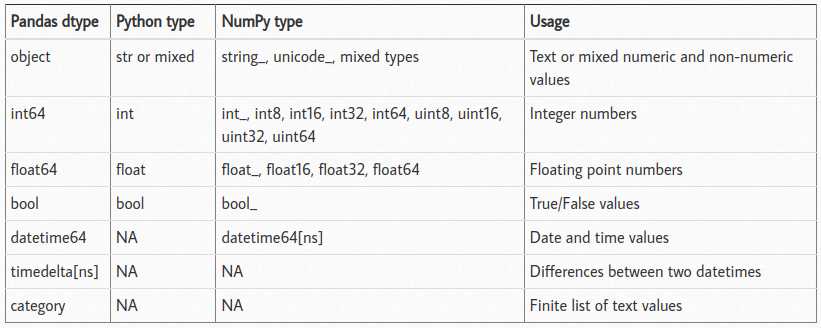
Python - Dataset Size
Index(['id', 'nome', 'localizacao', 'ano', 'quilometros_percorridos',
       'tipo_de_combustivel', 'transmissao', 'tipo_proprietario',
       'quilometragem_por_litro', 'motor', 'potencia', 'assentos',
       'novo_preco', 'preco'],
dtype='object')Python - Unique Values per Variable
id                         7253
nome                       2041
localizacao                  11
ano                          23
quilometros_percorridos    3660
tipo_de_combustivel           5
transmissao                   2
tipo_proprietario             4
quilometragem_por_litro     450
motor                       150
potencia                    386
assentos                      9
novo_preco                  625
preco                      1373
dtype: int64
Python - Null Values in Columns
id                            0
nome                          0
localizacao                   0
ano                           0
quilometros_percorridos       0
tipo_de_combustivel           0
transmissao                   0
tipo_proprietario             0
quilometragem_por_litro       2
motor                        46
potencia                     46
assentos                     53
novo_preco                 6247
preco                      1234
dtype: int64
Python - Removing Columns
# -----------------
# Remove 'id' column from the data
dados = dados.drop(columns = ['id'])
dados.info()
# -----------------
<class 'pandas.core.frame.DataFrame'>
RangeIndex: 7253 entries, 0 to 7252
Data columns (total 13 columns):
# Column Non-Null Count Dtype
--- ------ -------------- -----
0 nome 7253 non-null object
1 localizacao 7253 non-null object
2 ano 7253 non-null int64
3 quilometros_percorridos 7253 non-null int64
4 tipo_de_combustivel 7253 non-null object
5 transmissao 7253 non-null object
6 tipo_proprietario 7253 non-null object
7 quilometragem_por_litro 7251 non-null object
8 motor 7207 non-null object
9 potencia 7207 non-null object
10 assentos 7200 non-null float64
11 novo_preco 1006 non-null object
12 preco 6019 non-null float64
dtypes: float64(2), int64(2), object(9)
memory usage: 736.8+ KBPython - Summary Statistics
| ano | quilometros_percorridos | assentos | preco | |
|---|---|---|---|---|
| count | 7253.000000 | 7.253000e+03 | 7200.000000 | 6019.000000 |
| mean | 2013.365366 | 5.869906e+04 | 5.279722 | 9.479468 |
| std | 3.254421 | 8.442772e+04 | 0.811660 | 11.187917 |
| min | 1996.000000 | 1.710000e+02 | 0.000000 | 0.440000 |
| 25% | 2011.000000 | 3.400000e+04 | 5.000000 | 3.500000 |
| 50% | 2014.000000 | 5.341600e+04 | 5.000000 | 5.640000 |
| 75% | 2016.000000 | 7.300000e+04 | 5.000000 | 9.950000 |
| max | 2019.000000 | 6.500000e+06 | 10.000000 | 160.000000 |
NOTE: It only considers numeric data types and calculates metrics for types such as int and float.
Python - Measu. of Central Tendency
Calculating the mean in different ways:
Using Pandas
Using numpy
Python - Measu. of Central Tendency
Calculating the minimum in different ways:
Using Pandas
Using numpy
Python - Measu. of Central Tendency
Calculating quantiles:
Using Pandas
Using numpy
Why did numpy return nan?
Python - Measu. of Central Tendency
Calculating quantiles:
Using NumPy (Handling NaNs)
considering more than one quantile
array([ 0.44, 3.5 , 5.64, 9.95, 160. ])
Using pandas
Python - Measu. of Central Tendency
Calculating quantiles for multiple columns:
# -----------------
# Quantiles for multiple columns
# -----------------
dados[["quilometros_percorridos","preco"]].quantile([0,0.25,0.5,0.75,1]) #Pandas
# -----------------| quilometros_percorridos | preco | |
|---|---|---|
| 0.00 | 171.0 | 0.44 |
| 0.25 | 34000.0 | 3.50 |
| 0.50 | 53416.0 | 5.64 |
| 0.75 | 73000.0 | 9.95 |
| 1.00 | 6500000.0 | 160.00 |
Note: To avoid constantly showing more than one solution, we will focus on Pandas and stick with it until the end.
Python - Measures of Dispersion
Calculating variable variance:
ano                        1.059125e+01
quilometros_percorridos    7.128040e+09
assentos                   6.587914e-01
preco                      1.251695e+02
dtype: float64
Note: It considers numeric data types and calculates metrics as int, float.
Python - Measures of Dispersion
Calculating covariance between variables:
| ano | quilometros_percorridos | assentos | preco | |
|---|---|---|---|---|
| ano | 10.591255 | -5.161682e+04 | 0.021573 | 11.169366 |
| quilometros_percorridos | -51616.822165 | 7.128040e+09 | 6201.221577 | -11735.383472 |
| assentos | 0.021573 | 6.201222e+03 | 0.658791 | 0.473281 |
| preco | 11.169366 | -1.173538e+04 | 0.473281 | 125.169489 |
Note: It considers numeric data types and calculates metrics as int, float.
Python - Measures of Dispersion
Calculating correlation between variables:
# -----------------
dados.corr(numeric_only=True) # # Default is False and Pearson correlation
# -----------------| ano | quilometros_percorridos | assentos | preco | |
|---|---|---|---|---|
| ano | 1.000000 | -0.187859 | 0.008216 | 0.305327 |
| quilometros_percorridos | -0.187859 | 1.000000 | 0.090221 | -0.011493 |
| assentos | 0.008216 | 0.090221 | 1.000000 | 0.052225 |
| preco | 0.305327 | -0.011493 | 0.052225 | 1.000000 |
Note: It considers numeric data types and calculates metrics as int, float.
Python - Qualitative Variables
Calculating frequencies when variables are categorical
nome
Mahindra XUV500 W8 2WD                  55
Maruti Swift VDI                        49
Maruti Swift Dzire VDI                  42
Honda City 1.5 S MT                     39
Maruti Swift VDI BSIV                   37
                                        ..
Chevrolet Beat LT Option                 1
Skoda Rapid 1.6 MPI AT Elegance Plus     1
Ford EcoSport 1.5 TDCi Ambiente          1
Hyundai i10 Magna 1.1 iTech SE           1
Hyundai Elite i20 Magna Plus             1
Name: count, Length: 2041, dtype: int64
Python - Qualitative Variables
Calculating frequencies for categorical variables
# ---------------------
dados.groupby(["nome"])["nome"] \
      .count() \
      .reset_index(name='count') \
      .sort_values(['count'], ascending=False)
# ---------------------| nome | count | |
|---|---|---|
| 1017 | Mahindra XUV500 W8 2WD | 55 |
| 1265 | Maruti Swift VDI | 49 |
| 1241 | Maruti Swift Dzire VDI | 42 |
| 457 | Honda City 1.5 S MT | 39 |
| 1266 | Maruti Swift VDI BSIV | 37 |
| ... | ... | ... |
| 939 | Mahindra NuvoSport N8 | 1 |
| 937 | Mahindra Logan Petrol 1.4 GLE | 1 |
| 936 | Mahindra Logan Diesel 1.5 DLS | 1 |
| 935 | Mahindra KUV 100 mFALCON G80 K8 | 1 |
| 1020 | Mahindra Xylo D2 BS III | 1 |
2041 rows × 2 columns
Python - Qualitative Variables
Creating cross-tabulations between variables
Python - Qualitative Variables
Creating cross-tabulations between variables
Python - Qualitative Variables
Creating cross-tabulations between variables
# ---------------------
# Chi-Square Test with Transmission and Location
cross_tab = pd.crosstab(dados['transmissao'], dados['localizacao'])
# ---
c, p, dof, expected = chi2_contingency(cross_tab)
print(p)
# ---------------------1.3894902634085349e-55| localizacao | Ahmedabad | Bangalore | Chennai | Coimbatore | Delhi | Hyderabad | Jaipur | Kochi | Kolkata | Mumbai | Pune |
|---|---|---|---|---|---|---|---|---|---|---|---|
| transmissao | |||||||||||
| Automatic | 72 | 179 | 136 | 303 | 204 | 232 | 62 | 245 | 88 | 359 | 169 |
| Manual | 203 | 261 | 455 | 469 | 456 | 644 | 437 | 527 | 566 | 590 | 596 |
Python - Feature Creation
# -----------------
# Creating the 'idade_carro' variable as a new feature
from datetime import date
# ---
print("The current year is: " + str(date.today().year) )
# --
dados['idade_carro'] = date.today().year - dados['ano']
# --
dados[["nome", "preco", "ano", "idade_carro"]]
# -----------------
The current year is: 2026| nome | preco | ano | idade_carro | |
|---|---|---|---|---|
| 0 | Maruti Wagon R LXI CNG | 1.75 | 2010 | 16 |
| 1 | Hyundai Creta 1.6 CRDi SX Option | 12.50 | 2015 | 11 |
| 2 | Honda Jazz V | 4.50 | 2011 | 15 |
| 3 | Maruti Ertiga VDI | 6.00 | 2012 | 14 |
| 4 | Audi A4 New 2.0 TDI Multitronic | 17.74 | 2013 | 13 |
| ... | ... | ... | ... | ... |
| 7248 | Volkswagen Vento Diesel Trendline | NaN | 2011 | 15 |
| 7249 | Volkswagen Polo GT TSI | NaN | 2015 | 11 |
| 7250 | Nissan Micra Diesel XV | NaN | 2012 | 14 |
| 7251 | Volkswagen Polo GT TSI | NaN | 2013 | 13 |
| 7252 | Mercedes-Benz E-Class 2009-2013 E 220 CDI Avan... | NaN | 2014 | 12 |
7253 rows × 4 columns
Python - Variable Creation
# -----------------
# Creating the car 'marca' (brand) variable
# str.split: splits the strings
# str.get(0): gets the first element (index 0) from each list created per row
dados['marca'] = dados.nome.str.split().str.get(0)
# --
dados[['nome','marca']].head()
# -----------------| nome | marca | |
|---|---|---|
| 0 | Maruti Wagon R LXI CNG | Maruti |
| 1 | Hyundai Creta 1.6 CRDi SX Option | Hyundai |
| 2 | Honda Jazz V | Honda |
| 3 | Maruti Ertiga VDI | Maruti |
| 4 | Audi A4 New 2.0 TDI Multitronic | Audi |
NOTE: To return DataFrames with two or more selected columns, you must use double square brackets, i.e., df[[colname(s)]]. Single brackets return a Series, while double brackets return a DataFrame.
Python - Checking Variables
Before the charts, let’s check which variables are numerical and which are categorical.
# -----------------
cat_cols = dados.select_dtypes(include=['object']).columns
num_cols = dados.select_dtypes(include=np.number).columns.tolist()
print("Categorical Variables: " + str(cat_cols))
print("Numerical Variables: " + str(num_cols))
# -----------------
Categorical Variables: Index(['nome', 'localizacao', 'tipo_de_combustivel', 'transmissao',
'tipo_proprietario', 'quilometragem_por_litro', 'motor', 'potencia',
'novo_preco', 'marca'],
dtype='object')
Numerical Variables: ['ano', 'quilometros_percorridos', 'assentos', 'preco', 'idade_carro']Python - Plots
Histograms and BoxPlots
Python - Plots
Histograms and BoxPlots
ano
Skewness: -0.84
quilometros_percorridos
Skewness: 61.58
assentos
Skewness: 1.9
preco
Skewness: 3.34
idade_carro
Skewness: 0.84
Python - Plots
Bar Charts
# -----------------
fig, axes = plt.subplots(3, 2, figsize = (18, 18))
fig.suptitle('Bar Charts for all categorical variables in the dataset')
sns.countplot(ax = axes[0, 0], x = 'tipo_de_combustivel', data = dados, color = 'blue',
              order = dados['tipo_de_combustivel'].value_counts().index);
sns.countplot(ax = axes[0, 1], x = 'transmissao', data = dados, color = 'blue',
              order = dados['transmissao'].value_counts().index);
sns.countplot(ax = axes[1, 0], x = 'tipo_proprietario', data = dados, color = 'blue',
              order = dados['tipo_proprietario'].value_counts().index);
sns.countplot(ax = axes[1, 1], x = 'localizacao', data = dados, color = 'blue',
              order = dados['localizacao'].value_counts().index);
sns.countplot(ax = axes[2, 0], x = 'marca', data = dados, color = 'blue',
              order = dados['marca'].head(20).value_counts().index);
sns.countplot(ax = axes[2, 1], x = 'ano', data = dados, color = 'blue',
              order = dados['ano'].head(20).value_counts().index);
axes[1][1].tick_params(labelrotation=45);
axes[2][0].tick_params(labelrotation=90);
axes[2][1].tick_params(labelrotation=90);
# -----------------
Python - Plots
Bar Charts
# -----------------
sns.countplot( x = 'marca', data = dados, color = 'blue',
              order = dados['marca'].head(20).value_counts().index);
# -----------------
Python - Plots
Bivariate Plots
# -----------------
sns.pairplot(data=dados[['quilometros_percorridos','preco','transmissao']], \
             height=4.5, \
             corner = True,\
             hue="transmissao")
# -----------------
Python - Plots
Bivariate Plots

Python - Plots
Bar charts between categorical and numerical variables
Python - Plots
Bar Charts between Categorical and Numerical Variables
Text(0.5, 1.0, 'Transmission vs. Price')
Python - Plots
Bar Charts with two categorical and one numerical variable
# -------------------
# Creating a table for generating a plot distinct by categories
dfp = dados.pivot_table(index='ano', columns='transmissao', values='preco', aggfunc='mean')
# -------------------
dfp.head(10)
# -----------| transmissao | Automatic | Manual |
|---|---|---|
| ano | ||
| 1998 | 3.900000 | 0.610000 |
| 1999 | NaN | 0.835000 |
| 2000 | NaN | 1.175000 |
| 2001 | NaN | 1.543750 |
| 2002 | NaN | 1.294000 |
| 2003 | 11.305000 | 1.258000 |
| 2004 | 3.931667 | 1.463600 |
| 2005 | 4.467778 | 1.569167 |
| 2006 | 10.853636 | 2.124925 |
| 2007 | 6.825000 | 2.514286 |
Python - Plots
Bar charts for two categorical variables and one numerical variable

Python - Plots
Heatmap - Correlation Heatmap

Python - Other Visualization Libraries
- PlotLy - https://plotly.com/python/
Python - Other Visualization Libraries
Python - Other Visualization Libraries
- Plotnine - https://plotnine.readthedocs.io/en/stable/ - based on
ggplot2
Python - Other Visualization Libraries

Python - Report with SweetViz
Link: SWEETVIZ_REPORT.html
References
Basics
Aprendizado de Máquina: uma abordagem estatística, Izibicki, R. and Santos, T. M., 2020, link: https://rafaelizbicki.com/AME.pdf.
An Introduction to Statistical Learning: with Applications in R, James, G., Witten, D., Hastie, T. and Tibshirani, R., Springer, 2013, link: https://www.statlearning.com/.
Mathematics for Machine Learning, Deisenroth, M. P., Faisal. A. F., Ong, C. S., Cambridge University Press, 2020, link: https://mml-book.com.
References
Complementary
An Introduction to Statistical Learning: with Applications in python, James, G., Witten, D., Hastie, T. and Tibshirani, R., Taylor, J., Springer, 2023, link: https://www.statlearning.com/.
Matrix Calculus (for Machine Learning and Beyond), Paige Bright, Alan Edelman, Steven G. Johnson, 2025, link: https://arxiv.org/abs/2501.14787.
Machine Learning Beyond Point Predictions: Uncertainty Quantification, Izibicki, R., 2025, link: https://rafaelizbicki.com/UQ4ML.pdf.
Mathematics of Machine Learning, Petersen, P. C., 2022, link: http://www.pc-petersen.eu/ML_Lecture.pdf.
Machine Learning - Prof. Jodavid Ferreira