Statistical Machine Learning
Algorithmic Fairness and Bias Mitigation in Machine Learning
UFPE
Introduction to Fairness in ML
- Artificial Intelligence (AI) and Machine Learning (ML) algorithms are increasingly employed by businesses, governments, and organizations.
- They make decisions that have far-reaching impacts on individuals and society.
- High-stakes applications:
- Criminal justice (recidivism risk)
- Credit scoring and loan approval
- Hiring and human resources
- Medical diagnoses and resource allocation
Assumption: Algorithms are objective, mathematically pure, and immune to human prejudice.
Reality: Algorithms learn from historical data, inheriting, reflecting, and sometimes amplifying human biases.
The Brazilian AI Strategy (PBIA)
Context
The recently proposed Plano Brasileiro de Inteligência Artificial (PBIA) (https://www.gov.br/mcti/pt-br/centrais-de-conteudo/publicacoes-mcti/plano-brasileiro-de-inteligencia-artificial/pbia_mcti_2025.pdf) highlights the need for:
- AI for the Good of All (IA para o bem de todos): Focused on human well-being, social inclusion, and reducing inequalities.
- Centricity on Human Rights: Respecting dignity, diversity, and preventing discriminatory biases.
- Transparency and Accountability: Guaranteeing that AI processes are explainable, traceable, and responsible.
As data scientists and statisticians, we are the translators between these ethical guidelines and the mathematical optimization of predictive models.
What is Algorithmic Fairness?
Fairness in ML is the process of understanding, measuring, and mitigating algorithmic prejudice or favoritism toward people based on their sensitive characteristics.
- Individual Fairness: “Similar individuals should be treated similarly.” (Dwork et al., 2012)
- Group Fairness: Subgroups defined by protected attributes (e.g., race, gender) should receive similar outcomes or experience similar error rates.
Note: Fairness is not just a statistical issue; it is a dynamic, social, and legal construct.
Examples of Bias in Algorithms
Case Study 1: COMPAS (Criminal Justice)
The Context: COMPAS is a tool used in the US court system to predict the risk of a defendant re-offending (recidivism).
The Bias (ProPublica, 2016):
- In the algorithm was found a severe racial bias.
- Black defendants who did not re-offend were twice as likely to be incorrectly flagged as high risk (False Positives) compared to white defendants.
- White defendants who did re-offend were incorrectly labeled as low risk (False Negatives) more often than black defendants.
This violates the “Separation” fairness criteria (Equalized Odds).
Examples of Bias in Algorithms
Case Study 2: Amazon’s Recruiting Engine
The Context: Amazon built an AI tool to review job applicants’ resumes with the goal of automating the search for top talent.
The Bias:
- The models were trained on resumes submitted to the company over a 10-year period.
- Because the tech industry is male-dominated, the algorithm learned that male candidates were preferable.
- It penalized resumes that included words like “women’s” (e.g., “women’s chess club captain”) and downgraded graduates of two all-women’s colleges.
Amazon eventually had to scrap the project.
Examples of Bias in Algorithms
Case Study 3: Gender Shades (Computer Vision)
The Context: Commercial facial recognition systems provided by tech giants (IBM, Microsoft, Face++).
The Bias (Buolamwini & Gebru, 2018):
- Systems achieved 99% accuracy for lighter-skinned males.
- Accuracy dropped to 34.7% for darker-skinned females.
- Reason: The benchmark datasets used to train the algorithms (like Labeled Faces in the Wild) were overwhelmingly composed of lighter-skinned male faces.
This is a classic example of Representativeness Bias.
Types and Causes of Bias
Where Does Bias Come From?
Bias does not magically appear in algorithms; it enters through a socio-technical pipeline.
According to Ntoutsi et al. (2020), bias manifests via:
- Socio-technical causes: Human prejudices, institutional bias, and systemic inequalities existing in the real world.
- Data Generation & Collection: How we decide what to measure and who we sample.
- Model Training: The objective functions we choose to optimize (usually overall accuracy, ignoring minority group performance).
Types and Causes of Bias
Types of Data Bias
- Historical Bias: The data perfectly captures the world, but the world is flawed. (e.g., Amazon’s hiring tool).
- Representation Bias: Certain groups are under-represented or over-represented in the training data. (e.g., Gender Shades).
- Measurement Bias: How we define the target variable. Example: predicting “arrests” instead of “crimes committed” heavily biases against highly policed neighborhoods.
- Proxy Variables: Even if we drop the “Race” or “Gender” column, algorithms use correlated variables (like Zip Code, browsing history, or vocabulary) to recreate the sensitive attribute.
Types and Causes of Bias
The Danger of “Awareness through Blindness”
A common misconception among beginner data scientists:
“If I simply drop the ‘Race’ and ‘Gender’ columns from my dataset, the algorithm cannot be biased.”
Why this is mathematically false:
Due to multi-collinearity, highly non-linear algorithms (like Random Forests or Neural Networks) can reconstruct the protected attribute using latent combinations of other features (Redundant Encodings / Proxies).
To achieve fairness, we must often keep the sensitive variable during training to explicitly force the model not to use it, or to evaluate the bias post-training.
Protected Groups and Legal Concepts
What is a Protected Group?
A protected attribute (or sensitive attribute) is a demographic characteristic that cannot be legally or ethically used as the basis for a decision.
Common examples:
- Race / Ethnicity
- Gender / Sex
- Religion
- Age
- Sexual Orientation
- Disability status
We usually denote the sensitive attribute as \(A\), where \(A=a\) is the privileged group and \(A=b\) is the unprivileged group.
Protected Groups and Legal Concepts
Disparate Treatment vs. Disparate Impact
In legal frameworks (especially in the US and EU), discrimination is viewed through two lenses:
- Disparate Treatment (Direct Discrimination):
- The algorithm explicitly uses the protected attribute \(A\) to make a decision.
- Example: A rule that says
IF Gender == 'Female' THEN Credit_Limit = Lower.
- Disparate Impact (Indirect Discrimination):
- The algorithm uses seemingly neutral rules, but the outcome disproportionately harms a protected group.
- Example: A physical height requirement for a police force disproportionately excludes women.
Machine Learning naturally creates Disparate Impact if left unchecked.
Mathematical Metrics of Fairness
Notation and The Confusion Matrix
Let’s assume a binary classification problem:
- \(Y \in \{0,1\}\): Actual outcome (1 is favorable, e.g., Loan Granted).
- \(\hat{Y} \in \{0,1\}\): Predicted outcome.
- \(A \in \{a, b\}\): Protected attribute (\(a\) = privileged, \(b\) = unprivileged).
For any subgroup, we define standard metrics:
- TPR (True Positive Rate / Recall): \(P(\hat{Y}=1 | Y=1)\)
- FPR (False Positive Rate): \(P(\hat{Y}=1 | Y=0)\)
- PPV (Positive Predictive Value / Precision): \(P(Y=1 | \hat{Y}=1)\)
Fairness metrics compare these rates across groups \(a\) and \(b\).
Mathematical Metrics of Fairness
Statistical Parity (Independence)
Definition: The probability of a positive prediction should be identical across all groups. \[P(\hat{Y}=1 | A=a) = P(\hat{Y}=1 | A=b)\]
- Also known as Demographic Parity.
- Focuses entirely on the predicted outcome without looking at the true label \(Y\).
- Goal: Equal selection rates.
- Drawback: It might force the algorithm to select unqualified candidates in the unprivileged group just to meet the quota, reducing overall utility.
Mathematical Metrics of Fairness
Equal Opportunity (Relaxation of Separation)
Definition: The True Positive Rate (TPR) / Recall should be identical across groups. \[P(\hat{Y}=1 | Y=1, A=a) = P(\hat{Y}=1 | Y=1, A=b)\]
- Introduced by Hardt et al. (2016).
- Focuses on the qualified individuals.
- Goal: If you are actually a good candidate (\(Y=1\)), your chance of being selected (\(\hat{Y}=1\)) should not depend on your demographic group \(A\).
Mathematical Metrics of Fairness
Predictive Equality
Definition: The False Positive Rate (FPR) should be identical across groups. \[P(\hat{Y}=1 | Y=0, A=a) = P(\hat{Y}=1 | Y=0, A=b)\]
- Goal: The rate at which “bad” candidates are mistakenly given a favorable outcome should be equal.
- Alternatively, in a punitive setting (like predicting recidivism where 1 is “arrested”), this means innocent people should be falsely accused at the same rate across races.
Equalized Odds requires both Equal Opportunity (TPR) and Predictive Equality (FPR) to be satisfied simultaneously.
Mathematical Metrics of Fairness
Predictive Parity (Sufficiency)
Definition: The Positive Predictive Value (PPV) / Precision should be identical across groups. \[P(Y=1 | \hat{Y}=1, A=a) = P(Y=1 | \hat{Y}=1, A=b)\]
- Also known as Test Fairness or Calibration.
- Goal: If the algorithm predicts \(\hat{Y}=1\), the actual probability of success should be the same regardless of group.
- This is the metric the creators of the COMPAS algorithm argued they satisfied.
Mathematical Metrics of Fairness
The Impossibility Theorem of Fairness
Can we satisfy all these metrics at the same time? No.
Mathematical Proof (Chouldechova, 2017; Kleinberg et al., 2016): Unless the base rates (prevalence of \(Y=1\)) are exactly equal across groups \(a\) and \(b\), or the algorithm is a perfect predictor (100% accuracy), it is mathematically impossible to satisfy Separation (Equalized Odds) and Sufficiency (Predictive Parity) at the same time.
Implication for Statisticians: You must choose which fairness metric aligns best with the specific business, ethical, and legal context of your problem. There is no one-size-fits-all fairness.
Mathematical Metrics of Fairness
The Four-Fifths (80%) Rule
In practice, exact equality is impossible due to sample variance. How much difference is acceptable?
- The 80% Rule: Established by US Equal Employment Opportunity Commission (EEOC) in 1978, and used to detect disparate impact (potential discrimination).
- A selection rate for any group which is less than four-fifths (4/5 or 80%) of the rate for the highest group is regarded as evidence of adverse impact.
Mathematically, we accept bias if the ratio is within \([\epsilon, 1/\epsilon]\), where \(\epsilon = 0.8\): \[ 0.8 \le \frac{Metric_{unprivileged}}{Metric_{privileged}} \le 1.25 \]
Bias Mitigation Strategies
The Machine Learning Pipeline
Where can we intervene to fix bias?
- Pre-processing: Fix the data before feeding it to the algorithm.
- In-processing: Fix the algorithm so it learns fairly.
- Post-processing: Let the algorithm output whatever it wants, but fix the final predictions before deploying them.
Bias Mitigation Strategies
Pre-processing Methods
Modifying the training data distribution to remove underlying bias.
- Reweighting: Assigning different sample weights to instances. E.g., Give higher weight to unprivileged individuals with positive outcomes, and lower weight to privileged individuals with positive outcomes (Kamiran & Calders, 2011).
- Disparate Impact Remover: Editing feature values to preserve rank ordering but remove correlation with the sensitive attribute (Feldman et al., 2015).
- Optimized Pre-processing (Calmon et al., 2017): A probabilistic transformation that minimizes distortion of individual records while bounding discrimination and utility loss.
Bias Mitigation Strategies
In-processing Methods
Modifying the learning algorithm directly.
- Adversarial Debiasing: Training a Neural Network to predict \(Y\), while simultaneously training an “Adversary” network to predict \(A\) from the hidden layers. The main network is penalized if the adversary succeeds.
- Regularization: Adding a fairness penalty directly to the loss function (e.g., Logistic Regression with a constraint on Statistical Parity difference).
- Tree-based splits: Modifying the Gini impurity or Entropy criteria to also penalize splits that highly separate the protected groups.
Bias Mitigation Strategies
Post-processing Methods
Treating the model as a black box and modifying the threshold of the predictions.
- Cutoff Manipulation: Setting a different probability threshold for different groups. E.g., Threshold for Men = 0.6, Threshold for Women = 0.4. (Controversial legally, as it is explicit disparate treatment).
- Reject Option Classification (ROC Pivot): Focuses on instances near the decision boundary (high uncertainty). If an unprivileged person is just below the cutoff, promote them. If a privileged person is just above, demote them.
Introduction to the fairmodels Package
What is fairmodels?
fairmodels (Wiśniewski & Biecek) is an R package designed to:
- Easily calculate fairness metrics.
- Visualize biases across multiple models.
- Apply pre- and post-processing mitigation techniques.
It is built on top of DALEX (Descriptive mAchine Learning EXplanations), making it model-agnostic. It doesn’t matter if you used glm, ranger, xgboost, or tidymodels; fairmodels treats them all the same via an explainer object.
The Workflow in fairmodels
The standard 3-step pipeline:
- Train Model: Train any ML model in R.
- Create Explainer: Wrap the model, test data, and target variable using
DALEX::explain(). - Check Fairness: Pass the explainer, the protected attribute vector, and the privileged group name to
fairmodels::fairness_check().
Complete R Practical Session
Setup and The Dataset
We will use the German Credit Data (predicting credit risk: Good or Bad).
- Target:
Risk(1 = Good, 0 = Bad) - Sensitive Attribute:
Sex(Male vs Female) - Privileged Group: Male (historically favored in this dataset)
Complete R Practical Session
Step 1: Train Base Models
Let’s train a Logistic Regression and a Random Forest model.
Complete R Practical Session
Step 2: Create Explainers
We use DALEX to unify the prediction interface.
# Remove the target variable from the data passed to the explainer
X <- german[, -which(names(german) == "Risk")]

explainer_lm <- DALEX::explain(lm_model,
                        data = X,
                        y = y_numeric,
                        label = "Logistic Regression",
                        verbose = FALSE)

explainer_rf <- DALEX::explain(rf_model,
                        data = X,
                        y = y_numeric,
                        label = "Random Forest",
                        verbose = FALSE)
Complete R Practical Session
Step 3: Fairness Check
Now we evaluate if the models treat Males and Females differently.
Creating fairness classification object
-> Privileged subgroup : character ([32m Ok [39m )
-> Protected variable : factor ([32m Ok [39m )
-> Cutoff values for explainers : 0.5 ( for all subgroups )
-> Fairness objects : 0 objects
-> Checking explainers : 2 in total ( [32m compatible [39m )
-> Metric calculation : 10/13 metrics calculated for all models ( [33m3 NA created[39m )
[32m Fairness object created succesfully [39m
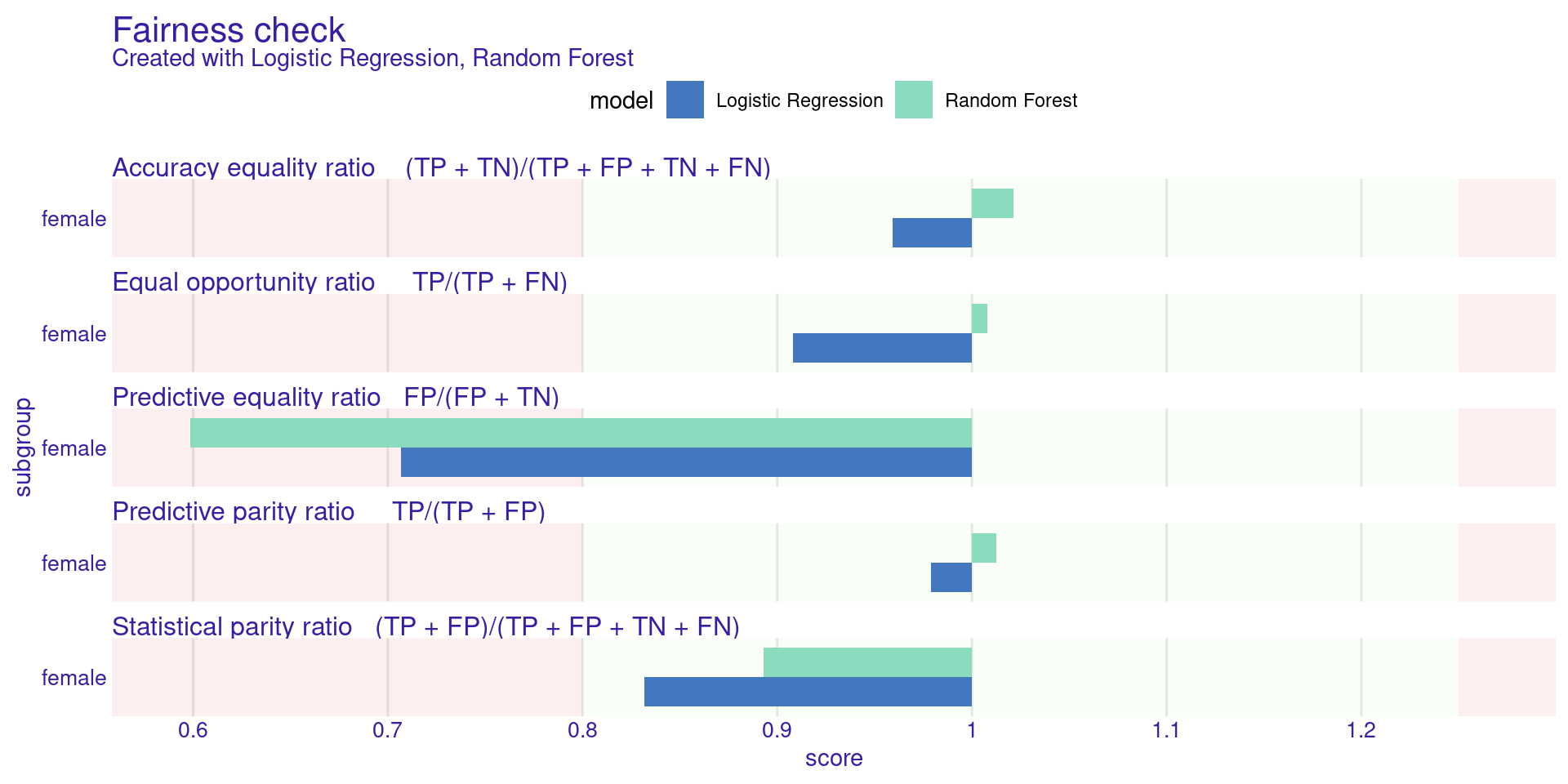
Fairness check for models: Logistic Regression, Random Forest
[33mLogistic Regression passes 4/5 metrics
[39mTotal loss : 0.6153324
[33mRandom Forest passes 4/5 metrics
[39mTotal loss : 0.5506964 Complete R Practical Session
Step 4: Visualizing Fairness (Parity Loss)
Parity Loss is calculated as taking the log of the metric ratio. If the ratio is perfectly 1, the log is 0 (Perfect fairness).
Complete R Practical Session
Step 4: Visualizing Fairness (Parity Loss)

Understanding the Plot:
- The plot shows colored bars for different metrics (Statistical Parity, Equal Opportunity, etc.).
- The green zone represents the “Acceptable Bias” area defined by \(\epsilon = 0.8\) (Ratio between 0.8 and 1.25).
- If a bar extends past the green zone, the model is significantly biased for that specific metric.
Complete R Practical Session
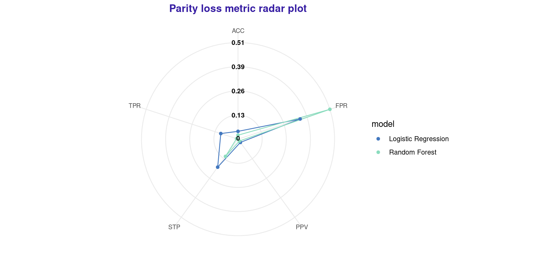
Step 4: Fairness Radar Plot
Another excellent way to visualize multiple metrics and compare models is the Radar Plot.
Complete R Practical Session
Step 4: Fairness Radar Plot

- In this plot, the center represents 0 parity loss (perfectly fair).
- The further out a point is, the more biased the model is in that metric.
- In this case, Random Forest is fairer than Logistic Regression in almost every aspect.
Complete R Practical Session
Step 5: Bias Mitigation (Pre-processing)
Let’s mitigate bias using Uniform Resampling. This duplicates unprivileged positive instances and removes privileged positive instances to balance the priors.
# Create a new debiased dataset
german_resampled <- german |>
  pre_process_data(protected = german$Sex,
                   y = y_numeric,
                   type = 'resample_uniform')

# Train a new model on the debiased data
lm_resampled <- glm(Risk ~ .,
                    data = german_resampled,
                    family = binomial(link = "logit"))

# Create new explainer
explainer_lm_resamp <- DALEX::explain(lm_resampled, data = X, y = y_numeric,
                               label = "LM_Resampled", verbose = FALSE)
Complete R Practical Session
Step 6: Bias Mitigation (Post-processing)
Alternatively, let’s try ROC Pivot (Reject Option Classification). We adjust the probabilities near the 0.5 threshold.
# Apply post-processing directly on the original explainer
explainer_rf_pivot <- explainer_rf |>
  roc_pivot(protected = german$Sex,
            privileged = "male",
            cutoff = 0.5, # critical region around 0.5
            theta = 0.05) # variable specifies maximal euclidean distance to cutoff resulting ing label switch

explainer_rf_pivot$label <- "RF_ROC_Pivot"
Complete R Practical Session
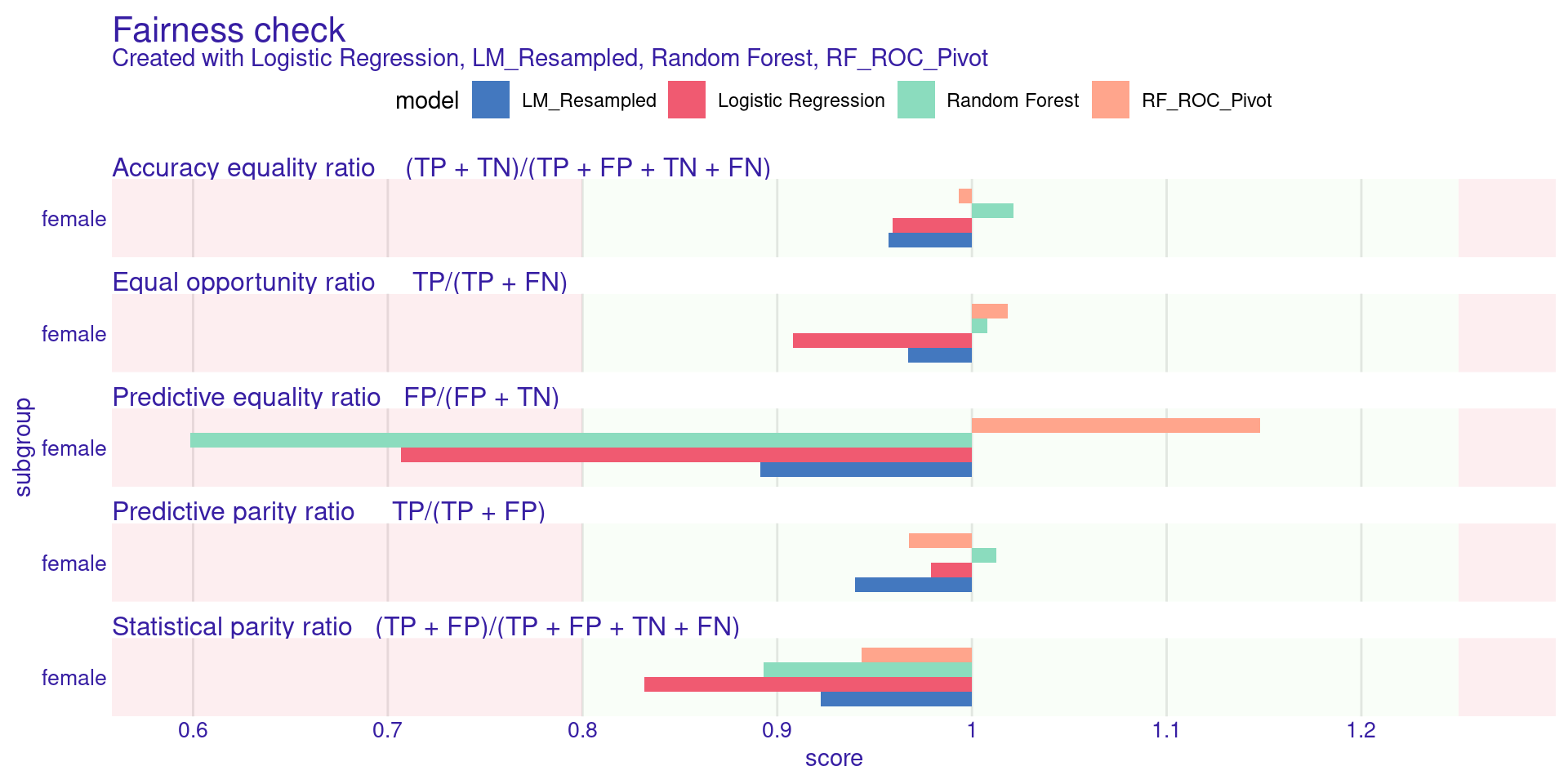
Step 7: Comparing Mitigated Models
Let’s put the original and the mitigated models side by side.
Creating fairness classification object
-> Privileged subgroup : character ([32m Ok [39m )
-> Protected variable : factor ([32m Ok [39m )
-> Cutoff values for explainers : 0.5 ( for all subgroups )
-> Fairness objects : 0 objects
-> Checking explainers : 4 in total ( [32m compatible [39m )
-> Metric calculation : 10/13 metrics calculated for all models ( [33m6 NA created[39m )
[32m Fairness object created succesfully [39m 
Complete R Practical Session
Step 7: Comparing Mitigated Models
What to expect:
The bars for LM_Resampled and RF_ROC_Pivot should be much smaller (closer to 0) and ideally fall within the green boundary, proving our mitigation strategies worked!
Trade-off: Accuracy vs. Fairness
Did we lose accuracy by forcing the models to be fair? We can check the performance and fairness trade-off.
Creating object with:
Fairness metric: TPR
Performance metric: accuracy 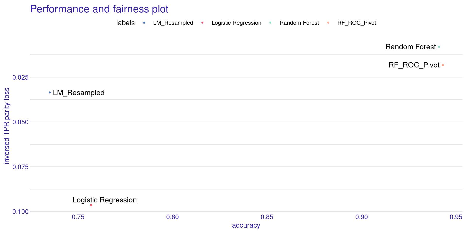
Trade-off: Accuracy vs. Fairness
Creating object with:
Fairness metric: TPR
Performance metric: accuracy 
- The X-axis shows Accuracy (Higher is better).
- The Y-axis shows inversed Parity Loss (Higher is better).
- The ideal model sits in the top-right corner.
- Usually, debiased models move slightly to the left (lose accuracy) but move drastically up (gain fairness).
Summary and Conclusion
Key Takeaways
- Bias is a socio-technical issue: Data records human history, including its flaws.
- Metrics conflict: You cannot satisfy Equal Opportunity and Predictive Parity simultaneously. You must choose based on context.
- Removing attributes is not enough: Proxies will leak protected information into the model.
- Mitigation is possible: Pre, In, and Post-processing techniques are mathematically robust ways to force models to adhere to ethical constraints.
- R is equipped for this: Using
DALEXandfairmodels, we can seamlessly audit and debug our models.
References
- Wiśniewski, J., & Biecek, P. (2022). fairmodels: a Flexible Tool for Bias Detection, Visualization, and Mitigation in Binary Classification Models. The R Journal.
- Calmon, F., et al. (2017). Optimized Pre-Processing for Discrimination Prevention. NeurIPS.
- Ntoutsi, E., et al. (2020). Bias in data-driven artificial intelligence systems—An introductory survey. WIREs Data Mining and Knowledge Discovery.
- PBIA (2024). Plano Brasileiro de Inteligência Artificial: IA para o bem de todos. MCTI / CGEE.
Statistical Machine Learning - Prof. Jodavid Ferreira