library(jpeg) # For reading JPEG images
library(tibble) # For creating data frames
library(dplyr) # For data manipulation
library(ggplot2) # For plotting

# Create a dummy image for demonstration if actual image is not present
# In a real scenario, you'd replace this with your actual image path
if (!file.exists("images/JODAVID.jpg")) {
  message("images/JODAVID.jpg not found. Creating a dummy image for demonstration.")
  # Create a simple image data (e.g., 50x50, 3 channels)
  dummy_image_data <- array(runif(50*50*3), dim = c(50, 50, 3))
  # Create the directory if it doesn't exist
  if (!dir.exists("Figures")) {
    dir.create("Figures")
  }
  # Save a simple JPEG image
  writeJPEG(dummy_image_data, "images/JODAVID.jpg")
}


# Read the image
imagem <- readJPEG("images/JODAVID.jpg")

# Organize the image into a data frame (long format)
# Each row represents a pixel with its (X,Y) coordinates and RGB values
imagemRGB <- tibble(
  X = rep(1:dim(imagem)[2], each = dim(imagem)[1]),
  Y = rep(dim(imagem)[1]:1, dim(imagem)[2]), # Y-axis inverted for plotting
  R = as.vector(imagem[,,1]),
  G = as.vector(imagem[,,2]),
  B = as.vector(imagem[,,3])
)Statistical Machine Learning
Clustering Methods
K-Means Visualization
Initial Data and Progression
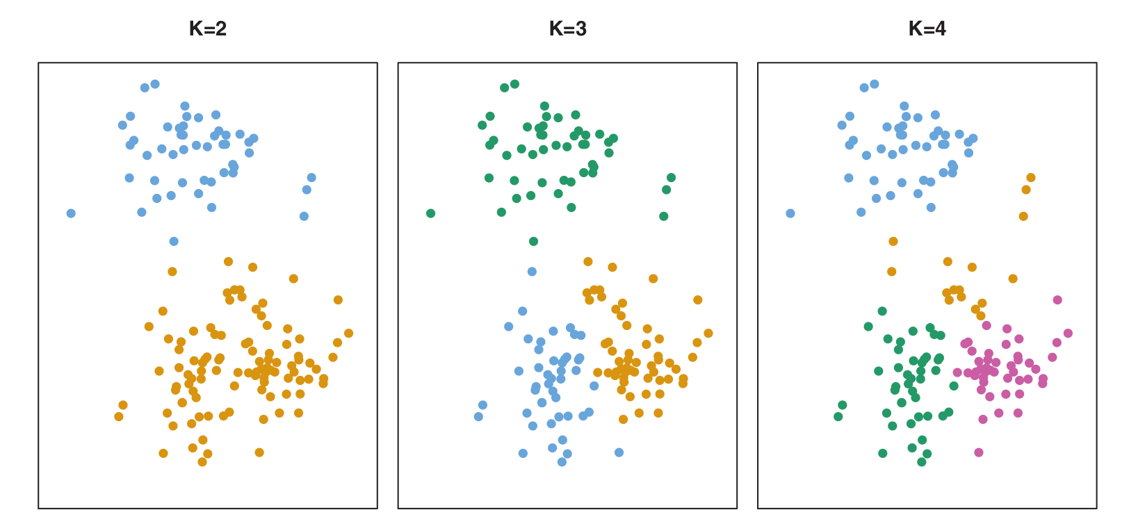
- Let’s visualize the K-Means algorithm with a simulated 2D dataset (\(n=150\)).
Figure (K=2, K=3, K=4): Shows how the clusters are formed for different values of \(K\).
K-Means Visualization
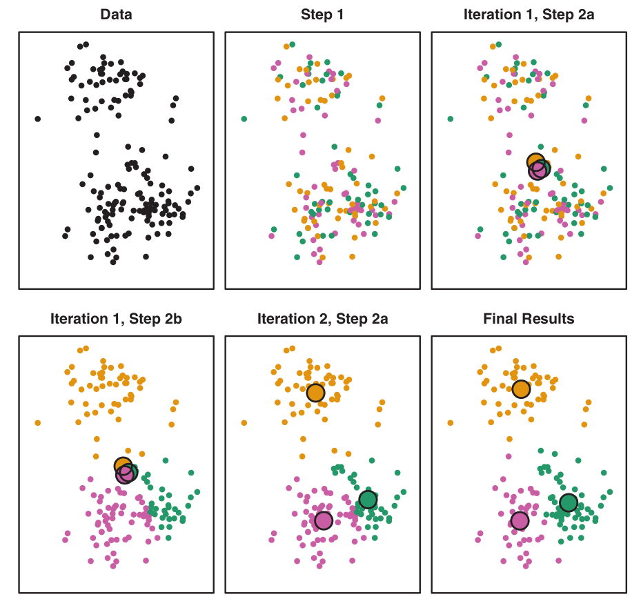
Algorithm Steps (K=3)
Figure: Illustrates the progression of K-Means algorithm for \(K=3\):
- Top left: Observations.
- Top center: Initial random assignment.
- Top right: Centroids computed.
- Bottom left: Observations reassigned.
- Bottom center: New centroids.
- Bottom right: Final result after 10 iterations.
K-Means Visualization
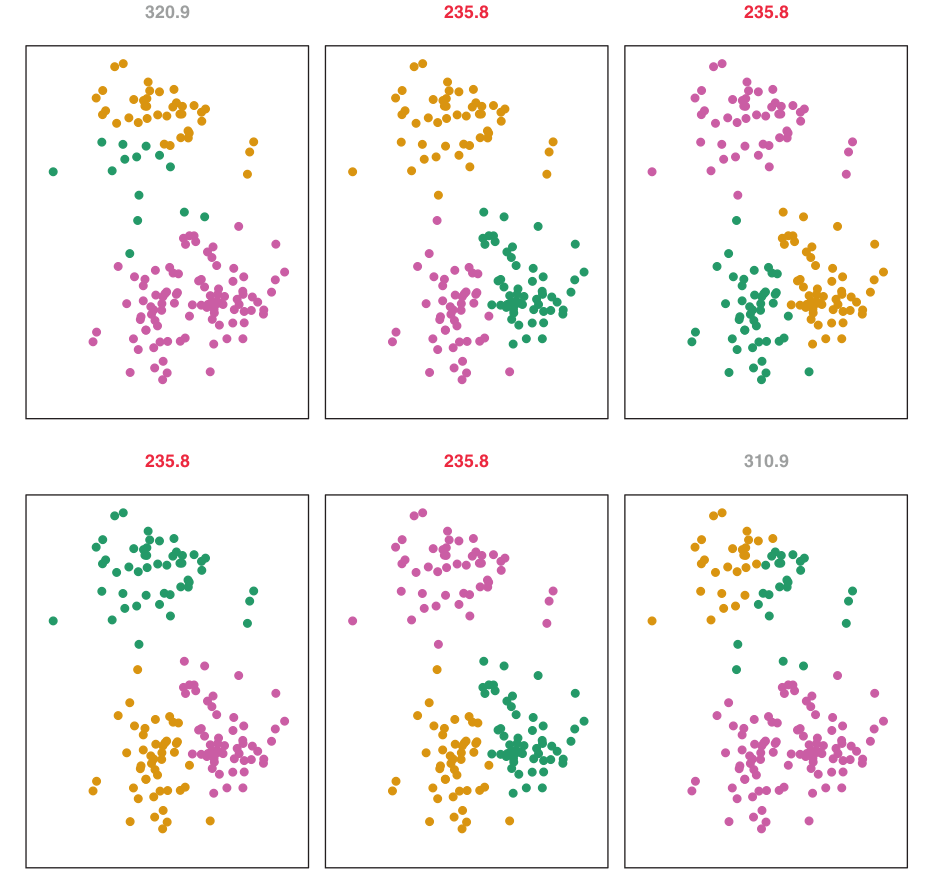
Multiple Initializations
Figure: K-Means clustering performed six times with different random initial assignments for \(K=3\).
- Values above each plot show the objective function.
- Multiple local optima are obtained. The best solution (lowest objective, \(235.8\)) provides better separation.
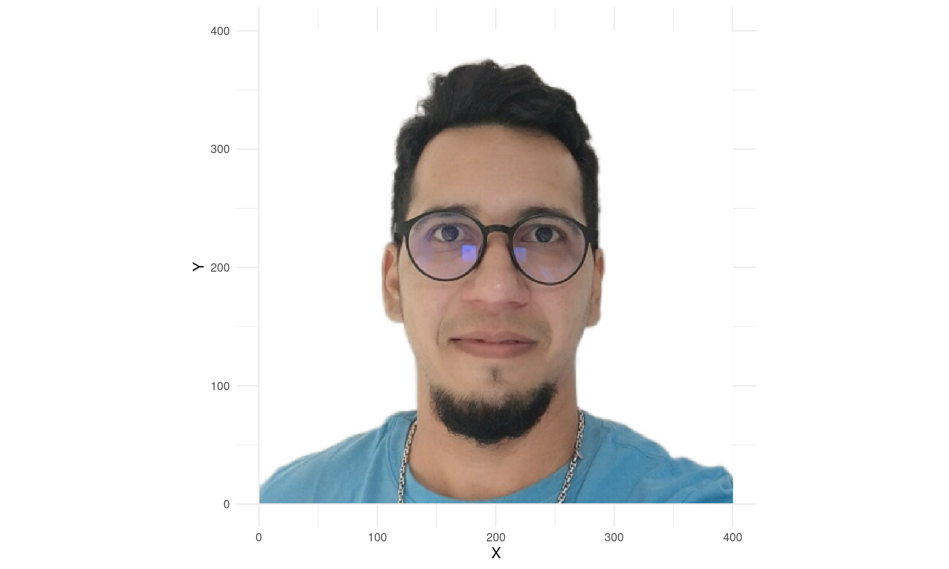
R Example: K-Means on Image Pixels
Code - Data Preparation
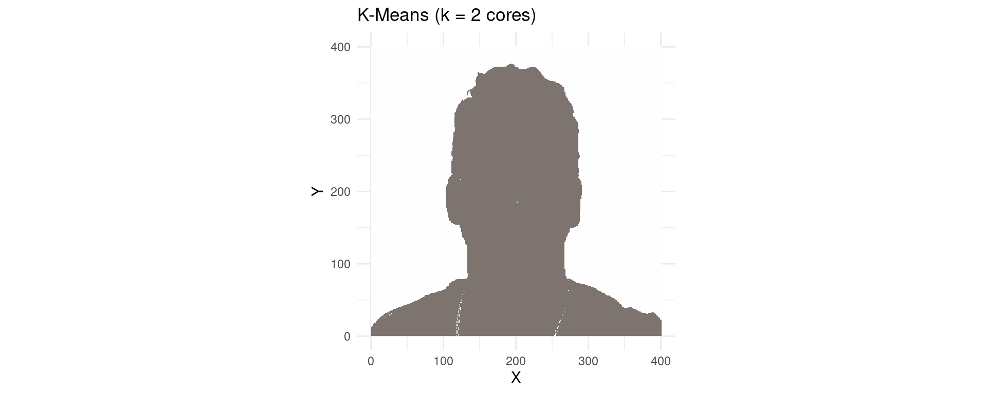
R Example: K-Means on Image Pixels
K-Means with K=2 Colors
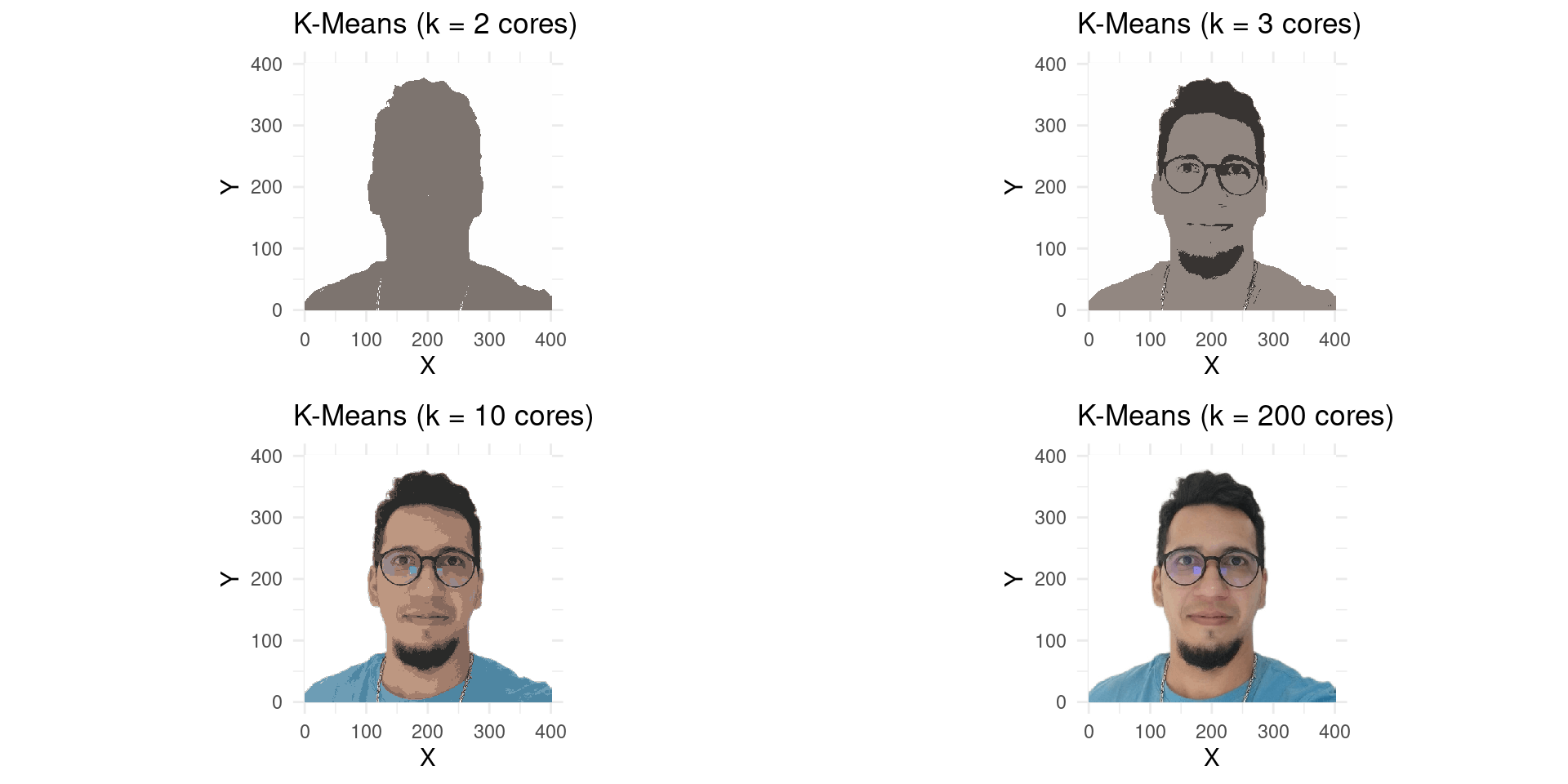
R Example: K-Means on Image Pixels
K-Means with differents Colors
The Elbow Method
Defining the Optimal K
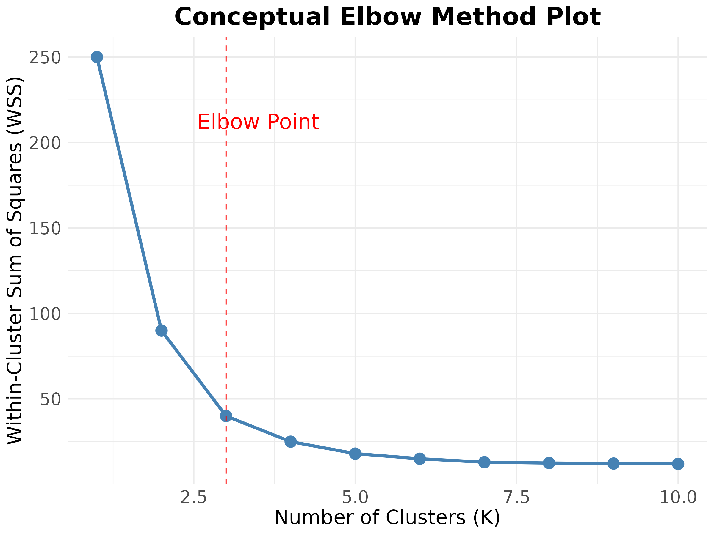
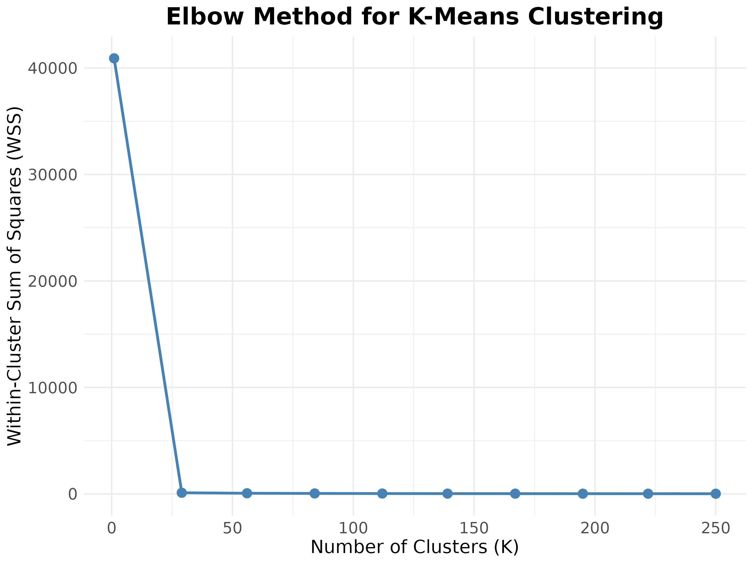
The Elbow method is a popular heuristic to help determine the optimal number of clusters (\(K\)) for the K-Means algorithm.
How it Works:
- It calculates the Within-Cluster Sum of Squares (WSS) for different values of \(K\) (e.g., from 1 to 10 or more).
- WSS measures the compactness of each cluster; the lower the WSS, the more compact the clusters.
- It then plots the WSS against \(K\).
The Elbow Method
Defining the Optimal K
Identifying the Ideal \(K\):
- As \(K\) increases, the WSS will always decrease (more clusters mean less dispersion within each).
- One looks for the point on the curve where the rate of decrease in WSS sharply changes and starts to ‘flatten out’ – this is the ‘elbow’.
- This point suggests that adding more clusters beyond this point does not provide a significant gain in the overall compactness of the clusters.
Considerations:
- It is a visual and subjective approach.
- A clear “elbow” may not always be apparent.
Example: Elbow Method
Practical Application - Jodavid Image
Example: Elbow Method
Practical Application - Jodavid Image

Interpreting a Dendrogram
Example Data
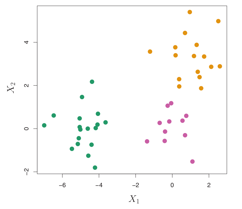
- Consider a simulated data set with 45 observations in 2D space, generated from a three-class model.
- The true class labels are shown in different colors, but we will treat them as unknown for clustering.
Figure:
- 45 observations in 2D space.
- Three distinct classes, shown in separate colors.
- We will seek to cluster the observations to discover these classes.
Interpreting a Dendrogram
Identifying Clusters
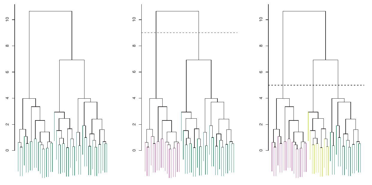
- To identify clusters from a dendrogram, we make a horizontal cut across the tree.
- The distinct sets of observations beneath the cut can be interpreted as clusters.
- The height of the cut serves the same role as \(K\) in K-Means clustering: it controls the number of clusters obtained.
Figure:
- Left: Dendrogram.
- Center: Cut at height 9, yielding two clusters.
- Right: Cut at height 5, yielding three clusters.
- Colors are for display, not used in clustering.
Interpreting a Dendrogram
Identifying Clusters
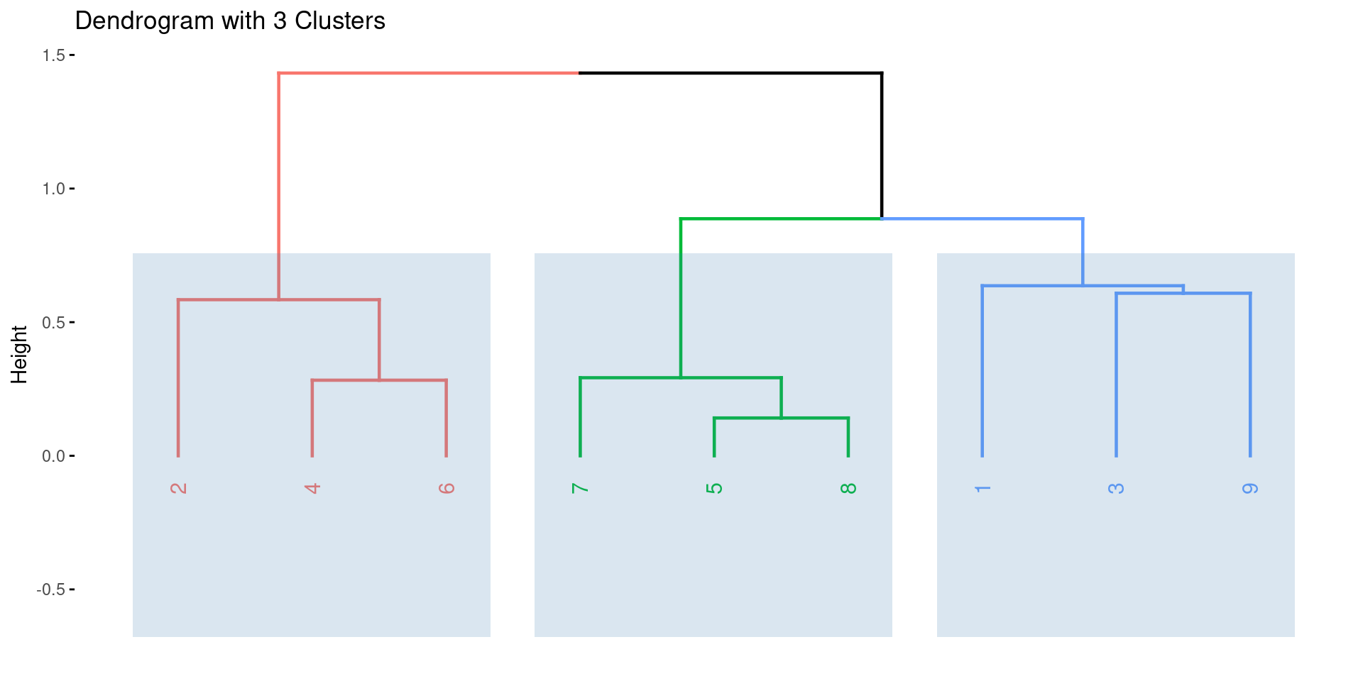
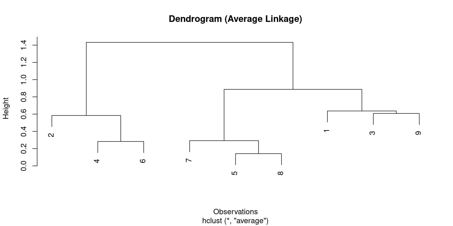
Interpreting a Dendrogram
Horizontal Axis Caution Example
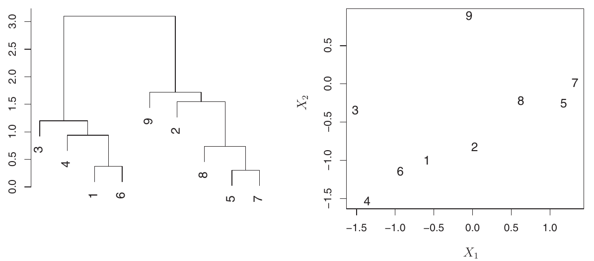
- Consider this dendrogram for 9 observations.
- Observations 5 and 7 are very similar (fuse low). Observations 1 and 6 are also similar.
- However, observations 9 and 2 are not necessarily similar just because they appear close horizontally. Their fusion height is higher.
Figure:
- Left: Dendrogram with 9 observations.
- Right: Raw data for these 9 observations.
- Confirms that horizontal proximity is misleading; vertical fusion height determines similarity.
Hierarchical Clustering
Linkage Type Impact
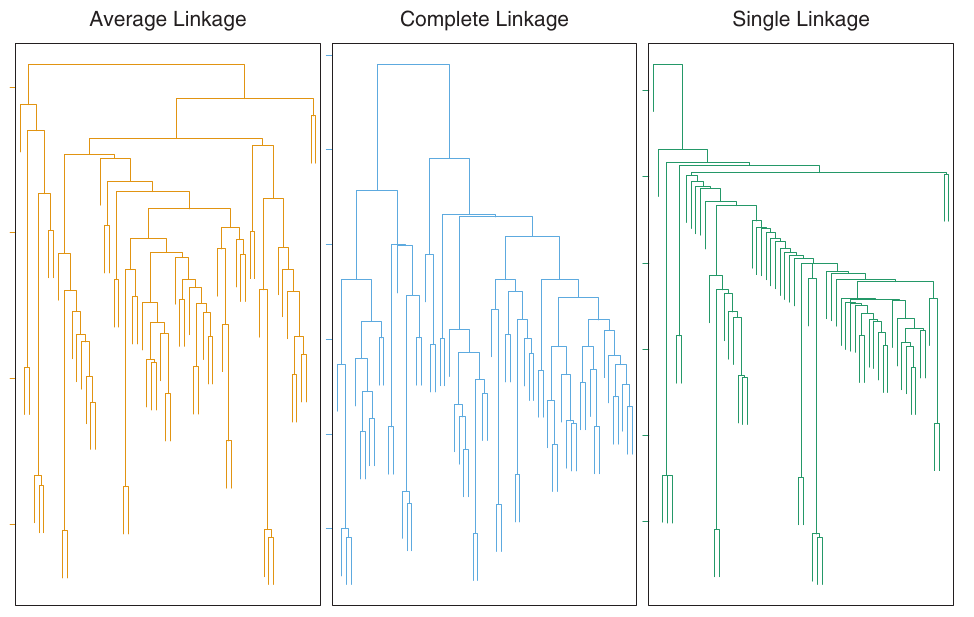
- Average, complete, and single linkage are most popular.
- Average and complete linkage are generally preferred as they tend to yield more balanced dendrograms.
- Centroid linkage can suffer from an inversion, where two clusters are fused at a height below either of the individual clusters in the dendrogram. This can hinder visualization and interpretation.
Figure:
- Shows how different linkage methods (Average, Complete, Single) applied to the same dataset produce different dendrogram structures.
- Average and Complete linkage tend to yield more balanced clusters.
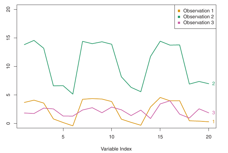
Choice of Dissimilarity Measure
Illustration
Figure:
- Three observations with 20 variables.
- Obs 1 & 3: Similar values, small Euclidean distance, weakly correlated, large correlation-based distance.
- Obs 1 & 2: Different values, large Euclidean distance, highly correlated, small correlation-based distance.
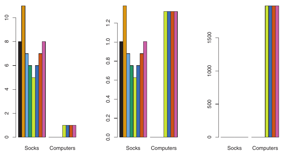
Scaling Variables
Illustration
If variables are scaled to have standard deviation one, each variable is given equal importance.
Also important when variables are measured on different scales (e.g., centimeters vs. kilometers). The choice of units can greatly affect the dissimilarity measure.
Figure:
- Left: Raw purchases (socks dominate).
- Center: Purchases scaled by standard deviation (computers now have greater relative effect).
- Right: Dollars spent (computers clearly dominate due to price).
- Clustering results will differ significantly based on these choices.
R Example: Hierarchical Clustering
Code - Hierarchical Clustering
- We will use
hclustfor hierarchical clustering andcutreeto obtain clusters. dist()calculates the distance matrix.
# A tibble: 9 × 4
     id    X1    X2 cluster_h
  <int> <dbl> <dbl>     <int>
1     1   0.1   0.4         1
2     2  -0.2  -0.3         2
3     3   0.5   0.9         1
4     4  -0.8  -0.7         2
5     5   0.7   0.1         3
6     6  -0.6  -0.5         2
7     7   0.8   0.3         3
8     8   0.6   0           3
9     9  -0.1   1           1
R Example: Hierarchical Clustering
Dendrogram Visualization
- The plot generated by
plot(dendrograma)is the standard R dendrogram.
R Example: Hierarchical Clustering
Enhanced Visualization with factoextra
- The
factoextrapackage provides excellent tools for visualizing clustering results, including dendrograms with enhanced features.

R Example: Hierarchical Clustering
Dendrogram with 3 Clusters