Statistical Machine Learning
Classification Methods
UFPE
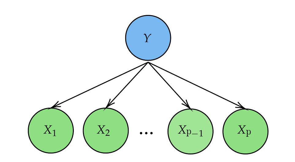
Notation
- \(X\) or \(Y\)
- \(x\) or \(y\)
- \(\mathbf{x}\) or \(\mathbf{y}\)
- \(\dot{\mathbf{x}}\) or \(\dot{\mathbf{y}}\)
- \(\mathbf{X}\) or \(\mathbf{Y}\)
- \(\dot{\mathbf{X}}\) or \(\dot{\mathbf{Y}}\)
- \(p\)
- \(n\)
- \(i\)
- \(j\)
- \(K\)
- \(k\)
represent random variables (r.v.);
represent realizations of random variables;
represent random vectors;
represent realizations of random vectors;
represent random matrices;
represent realizations of random matrices;
dimension of features, variables, parameters;
sample size;
\(i\)-th observation, instance (e.g., \(i=1, ..., n\));
\(j\)-th feature, variable, parameter (e.g., \(j=1, ..., p\));
number of classes (i.e., cardinality of class set \(\mathcal{C}\));
number of folds in CV / number of nearest neighbors in \(k\)-NN.
Remembering: Risk Function
- Assume \(Y\) takes values in a finite set of classes \(\mathcal{C}\) (e.g., \(\mathcal{C} = \{0, 1\}\) or \(\mathcal{C} = \{\text{spam, not spam}\}\)).
- The regression risk function \(R(f) = \mathbb{E}[(Y - f(\mathbf{x}))^2]\) is not suitable for classification (since classes are categorical, the difference \(Y - f(\mathbf{x})\) is not defined).
- A standard risk function for classification is based on the 0-1 loss:
\[R(f) := \mathbb{E}[I(Y \neq f(\mathbf{x}))] = P(Y \neq f(\mathbf{x}))\]
- This represents the probability of misclassification.
- The corresponding loss function is:
\[L(f(\mathbf{x}), Y) = I(Y \neq f(\mathbf{x}))\]
Optimal Classifier
- In regression, the function that minimizes the squared error risk is the regression function \(\hat{f}(\dot{\mathbf{x}}) = \mathbb{E}[Y|\mathbf{x}=\dot{\mathbf{x}}]\).
- For classification, the function \(\hat{f}\) that minimizes the 0-1 risk is given by: \[\hat{f}(\dot{\mathbf{x}}) = \underset{c \in \mathcal{C}}{\text{arg max }} P(Y=c|\mathbf{x}=\dot{\mathbf{x}})\]
- This means a realized feature vector \(\dot{\mathbf{x}}\) should be classified to the class \(c\) with the highest posterior (conditional) probability.
- This optimal classifier \(\hat{f}\) is known as the Bayes classifier.
- Like \(\mathbb{E}[Y|\mathbf{x}=\dot{\mathbf{x}}]\) in regression, the conditional probability \(P(Y=c|\mathbf{x}=\dot{\mathbf{x}})\) is generally unknown in practice and must be estimated from data.
Bayes Classifier
Theorem: Suppose we define the risk of a prediction function \(\hat{f}: \mathbb{R}^p \to \mathcal{C}\) via 0-1 loss: \(R(\hat{f}) = P(Y \neq \hat{f}(\mathbf{x}))\), where \((\mathbf{x},Y)\) is a new draw from the joint distribution.
Then the function \(\hat{f}\) that minimizes \(R(\hat{f})\) is given by:
\[\hat{f}(\dot{\mathbf{x}}) = \underset{c \in \mathcal{C}}{\text{arg max }} P(Y=c|\mathbf{x}=\dot{\mathbf{x}})\]
Demonstration - Binary Case
- Assume \(Y\) takes two values, \(c_1\) and \(c_2\) (binary classification problem).
\[\begin{align} R(\hat{f}) = & \mathbb{E}[I(Y \neq \hat{f}(\mathbf{x}))] = P(Y \neq \hat{f}(\mathbf{x})) \\ = & \int_{\mathbb{R}^p} P(Y \neq \hat{f}(\dot{\mathbf{x}})|\mathbf{x}=\dot{\mathbf{x}}) p(\dot{\mathbf{x}}) d\dot{\mathbf{x}} \\ = & \int_{\mathbb{R}^p} [I(\hat{f}(\dot{\mathbf{x}})=c_2)P(Y=c_1|\mathbf{x}=\dot{\mathbf{x}}) + \\ & I(\hat{f}(\dot{\mathbf{x}})=c_1)P(Y=c_2|\mathbf{x}=\dot{\mathbf{x}})] p(\dot{\mathbf{x}}) d\dot{\mathbf{x}} \end{align}\]
where \(p(\dot{\mathbf{x}})\) is the probability density function of \(\mathbf{x}\).
Bayes Classifier for Binary Case
- To minimize the overall risk \(R(\hat{f})\), we can minimize the term in the square brackets for each fixed realization \(\dot{\mathbf{x}}\):
- If we set \(\hat{f}(\dot{\mathbf{x}}) = c_1\), the term is \(P(Y=c_2|\mathbf{x}=\dot{\mathbf{x}})\).
- If we set \(\hat{f}(\dot{\mathbf{x}}) = c_2\), the term is \(P(Y=c_1|\mathbf{x}=\dot{\mathbf{x}})\).
- Thus, we minimize the error by choosing \(\hat{f}(\dot{\mathbf{x}})=c_1\) when \(P(Y=c_1|\mathbf{x}=\dot{\mathbf{x}}) \ge P(Y=c_2|\mathbf{x}=\dot{\mathbf{x}})\), and \(\hat{f}(\dot{\mathbf{x}})=c_2\) otherwise.
- For the binary case, the Bayes classifier can be rewritten as:
\[ \hat{f}(\dot{\mathbf{x}}) = c_1 \iff P(Y=c_1|\mathbf{x}=\dot{\mathbf{x}}) \ge \frac{1}{2} \]
- Observation: In binary classification, it is common to denote classes in \(\mathcal{C}\) as 0 and 1. This is arbitrary and doesn’t imply an ordering.
Bayes Error Rate
- The risk of the Bayes classifier, \(R(\hat{f})\), is called the Bayes error rate (or irreducible error rate):
\[ R(\hat{f}) = 1 - \mathbb{E}\left[ \max_{c \in \mathcal{C}} P(Y=c | \mathbf{x}) \right] \]
- For a binary classification problem (\(Y \in \{c_1, c_2\}\)), this simplifies to:
\[ R(\hat{f}) = \mathbb{E}\left[ \min\left( P(Y=c_1 | \mathbf{x}), P(Y=c_2 | \mathbf{x}) \right) \right] \]
- The Bayes error rate is the minimum possible error rate that any classifier can achieve on the population. It plays a role analogous to the variance of the error term \(\sigma^2\) in regression.
Model Selection
- To select a model \(\hat{f}\) from a class of candidate models \(\mathcal{G}\):
- Use cross-validation (or a validation set) to estimate \(R (\hat{f})\) for each \(\hat{f} \in \mathcal{G}\).
- Choose the model \(\hat{\tilde{f}}\) with the smallest estimated validation risk \(\tilde{R} (\hat{f})\).
- The following theorem provides a theoretical guarantee that this procedure likely returns a model close to the best available in \(\mathcal{G}\).
Model Selection Guarantee
Theorem: Let \(\mathcal{G} = \{\hat{f}_1, \dots, \hat{f}_T\}\) be a finite class of \(T\) candidate classifiers estimated from a training set. Let \(\tilde{R}(\hat{f})\) be the estimated error of \(\hat{f}\) on an independent validation set of size \(m = n - s\). Let \(\hat{f}^*\) be the model that minimizes the true risk \(R(\hat{f})\) among \(\hat{f} \in \mathcal{G}\), and let \(\hat{\tilde{f}}\) be the model that minimizes the estimated validation risk \(\tilde{R}(\hat{f})\) among \(\hat{f} \in \mathcal{G}\).
Then, for any \(\epsilon > 0\), with probability at least \(1-\epsilon\): \[ R(\hat{\tilde{f}}) \le R(\hat{f}^*) + 2 \sqrt{\frac{1}{2m} \log \frac{2T}{\epsilon}} \]
Implications of the Theorem
- The larger the number of classifiers \(T\) in \(\mathcal{G}\), the looser the bound (we need a larger validation set \(m\) to maintain the same guarantee).
- This motivates comparing only a small set of final candidate models on the test set.
- Tuning of each model (e.g., hyperparameter selection) should be done using cross-validation.
- The final test set must be reserved solely for comparing the best model from each class of models (e.g., best logistic regression vs. best \(k\)-NN) to prevent selection bias (optimism bias).
Plug-in Classifiers
Plug-in Classifiers
- The definition of the Bayes classifier suggests a simple approach for prediction:
- Estimate the posterior probabilities \(P(Y=c|\mathbf{x}=\dot{\mathbf{x}})\) for each category \(c \in \mathcal{C}\) from data.
- Then, define the classifier by plugging in these estimates: \[\hat{f}(\dot{\mathbf{x}}) = \underset{c \in \mathcal{C}}{\text{arg max }} \hat{P}(Y=c|\mathbf{x}=\dot{\mathbf{x}})\]
- For the binary case: \(\hat{f}(\dot{\mathbf{x}}) = 1 \iff \hat{P}(Y=1|\mathbf{x}=\dot{\mathbf{x}}) > 1/2\).
- This approach is known as a plug-in classifier because we “plug in” an estimator of the conditional probability into the formula for the optimal classifier.
- Thus, creating a classifier boils down to estimating \(P(Y=c|\mathbf{x}=\dot{\mathbf{x}})\).
Generative vs.
Discriminative Classifiers
Plug-in classifiers generally fall into two main paradigms:
- Discriminative Classifiers:
- Directly model the conditional distribution \(P(Y=c|\mathbf{x}=\dot{\mathbf{x}})\) without modeling the marginal feature distribution.
- Examples: Logistic Regression, \(k\)-Nearest Neighbors, Decision Trees.
- Generative Classifiers:
- Model the class-conditional density \(p(\dot{\mathbf{x}}|Y=c)\) and the prior probability \(P(Y=c)\). Compute the posterior probability using Bayes’ Theorem: \[ P(Y=c|\mathbf{x}=\dot{\mathbf{x}}) = \frac{p(\dot{\mathbf{x}}|Y=c)P(Y=c)}{\sum_{s \in \mathcal{C}} p(\dot{\mathbf{x}}|Y=s)P(Y=s)} \]
- Examples: Naive Bayes, Linear Discriminant Analysis (LDA), Quadratic Discriminant Analysis (QDA).
Regression Methods for Classification
- Note that for any \(c \in \mathcal{C}\), \(P(Y=c|\mathbf{x}=\dot{\mathbf{x}}) = \mathbb{E}[I(Y=c)|\mathbf{x}=\dot{\mathbf{x}}]\).
- Let \(Z_c = I(Y=c)\). We can use any regression model (trees, forests, linear models, etc.) to estimate the conditional expectation \(\mathbb{E}[Z_c|\mathbf{x}=\dot{\mathbf{x}}]\).
- Example: Linear regression to estimate \(P(Y=c|\mathbf{x}=\dot{\mathbf{x}})\): \[ P(Y=c|\mathbf{x}=\dot{\mathbf{x}}) = \mathbb{E}[Z_c|\mathbf{x}=\dot{\mathbf{x}}] \approx \beta_0^{(c)} + \beta_1^{(c)}\dot{x}_1 + \dots + \beta_p^{(c)}\dot{x}_p = (\boldsymbol{\beta}^{(c)})^\top \dot{\mathbf{x}} \] where \(\dot{\mathbf{x}} = (1, \dot{x}_1, \dots, \dot{x}_p)^\top\) and \(\boldsymbol{\beta}^{(c)} = (\beta_0^{(c)}, \beta_1^{(c)}, \dots, \beta_p^{(c)})^\top\).
- Coefficients can be estimated using Ordinary Least Squares (OLS), etc.
- Drawback: Estimated probabilities \(\hat{P}(Y=c|\mathbf{x}=\dot{\mathbf{x}})\) can lie outside the interval \([0, 1]\).
- This motivates models like logistic regression which naturally constrain probabilities to \([0,1]\).
Logistic Regression
- Assume \(Y\) is binary, \(\mathcal{C}=\{0,1\}\). Two classes are often denoted as “class 0” (0) and “class 1” (1).
- Logistic regression models \(P(Y=1|\mathbf{x}=\dot{\mathbf{x}})\) using the logistic (sigmoid) function: \[ P(Y=1|\mathbf{x}=\dot{\mathbf{x}}) = \frac{e^{\boldsymbol{\beta}^\top \dot{\mathbf{x}}}}{1 + e^{\boldsymbol{\beta}^\top \dot{\mathbf{x}}}} = \frac{1}{1 + e^{-\boldsymbol{\beta}^\top \dot{\mathbf{x}}}} \] where \(\boldsymbol{\beta} = (\beta_0, \beta_1, \dots, \beta_p)^\top\) and \(\dot{\mathbf{x}} = (1, \dot{x}_1, \dots, \dot{x}_p)^\top\).
Equivalently, the model assumes a linear relationship for the log-odds (logit): \[ \log \left( \frac{P(Y=1|\mathbf{x}=\dot{\mathbf{x}})}{1 - P(Y=1|\mathbf{x}=\dot{\mathbf{x}})} \right) = \boldsymbol{\beta}^\top \dot{\mathbf{x}} = \beta_0 + \beta_1 \dot{x}_1 + \dots + \beta_p \dot{x}_p \]
We do not assume this relationship is perfectly true in nature, but we use it as a parametric approximation to build a classifier.
Logistic Regression
Estimating Coefficients via MLE
Coefficients \(\boldsymbol{\beta}\) are estimated using Maximum Likelihood Estimation (MLE).
Given i.i.d. observations \((\dot{\mathbf{x}}_i, y_i)_{i=1}^n\), the conditional likelihood function is: \[ L(\boldsymbol{\beta}; \dot{\mathbf{y}}, \dot{\mathbf{X}}) = \prod_{i=1}^n [p_i(\boldsymbol{\beta})]^{y_i} [1 - p_i(\boldsymbol{\beta})]^{1-y_i} \] where \(p_i(\boldsymbol{\beta}) = P(Y_i=1|\mathbf{x}_i=\dot{\mathbf{x}}_i, \boldsymbol{\beta}) = \frac{1}{1 + e^{-\boldsymbol{\beta}^\top \dot{\mathbf{x}}_i}}\).
Maximizing the likelihood is equivalent to maximizing the log-likelihood: \[ \ell(\boldsymbol{\beta}) = \sum_{i=1}^n \left[ y_i \log p_i(\boldsymbol{\beta}) + (1-y_i) \log(1 - p_i(\boldsymbol{\beta})) \right] = \sum_{i=1}^n \left[ y_i \boldsymbol{\beta}^\top \dot{\mathbf{x}}_i - \log(1 + e^{\boldsymbol{\beta}^\top \dot{\mathbf{x}}_i}) \right] \]
Since there is no closed-form solution for \(\hat{\boldsymbol{\beta}}\), numerical optimization (e.g., Newton-Raphson or Iteratively Reweighted Least Squares - IRLS) is used.
Multi-class Logistic Regression
When the number of classes \(K = |\mathcal{C}| > 2\):
Multinomial Logistic Regression (Softmax Regression): Directly models the multi-class probabilities using: \[ P(Y=c|\mathbf{x}=\dot{\mathbf{x}}) = \frac{e^{\boldsymbol{\beta}_c^\top \dot{\mathbf{x}}}}{\sum_{s \in \mathcal{C}} e^{\boldsymbol{\beta}_s^\top \dot{\mathbf{x}}}} \] To ensure identifiability, one class is chosen as a reference (e.g., \(c_{ref}\)), setting \(\boldsymbol{\beta}_{c_{ref}} = \mathbf{0}\).
One-vs-Rest (OvR):
- Fits \(K\) separate binary logistic regression models, comparing each class \(c\) against all other classes combined.
- Classifies a new point to the class that yields the highest predicted probability: \[ \hat{f}(\dot{\mathbf{x}}) = \underset{c \in \mathcal{C}}{\text{arg max }} \hat{P}(Y=c | \mathbf{x} = \dot{\mathbf{x}}) \]
Naive Bayes
- Another approach to estimate \(P(Y=c|\mathbf{x}=\dot{\mathbf{x}})\) uses Bayes’ Theorem directly (Generative approach):
\[ P(Y=c|\mathbf{x}=\dot{\mathbf{x}}) = \frac{p(\dot{\mathbf{x}}|Y=c)P(Y=c)}{\sum_{s \in \mathcal{C}} p(\dot{\mathbf{x}}|Y=s)P(Y=s)} \]
- To calculate this, we need to estimate:
- Marginal class probabilities (priors) \(P(Y=c)\):
- Can be estimated directly from the sample proportions: \(\hat{P}(Y=c) = \frac{n_c}{n}\), where \(n_c = \sum_{i=1}^n I(y_i = c)\).
- Class-conditional densities \(p(\dot{\mathbf{x}}|Y=c)\):
- The joint distribution of the features given the class.
- Marginal class probabilities (priors) \(P(Y=c)\):
The “Naive” Assumption
- Estimating \(p(\dot{\mathbf{x}}|Y=c)\) for a high-dimensional vector \(\dot{\mathbf{x}} = (\dot{x}_1, \dots, \dot{x}_p)^\top\) is difficult due to the curse of dimensionality.
The Naive Bayes classifier simplifies this by making the “naive” assumption that features are conditionally pairwise independent given the class: \[ p(\dot{\mathbf{x}}|Y=c) = p((\dot{x}_1, \dots, \dot{x}_p)|Y=c) = \prod_{j=1}^p p_j(\dot{x}_j|Y=c) \]
This assumption is often unrealistic in practice, yet Naive Bayes frequently yields competitive classification performance.
Under this assumption, we only need to estimate \(p\) univariate densities \(p_j(\dot{x}_j|Y=c)\) for each class.
- For continuous features, we can be assume \(X_j|Y=c \sim N(\mu_{j,c}, \sigma^2_{j,c})\), that is “Gaussian Naive Bayes”.
Naive Bayes
Implementation Details
- If we assume \(X_j|Y=c \sim N(\mu_{j,c}, \sigma^2_{j,c})\), parameters are estimated via MLE:
- \(\hat{\mu}_{j,c} = \frac{1}{n_c} \sum_{i \in C_c} x_{ij}\)
- \(\hat{\sigma}^2_{j,c} = \frac{1}{n_c} \sum_{i \in C_c} (x_{ij} - \hat{\mu}_{j,c})^2\) where \(C_c = \{i : y_i = c\}\) and \(n_c = |C_c|\).
- For discrete features, \(P(X_j = v | Y=c)\) is estimated using frequency counts.
- Numerical Stability (Log-sum-exp trick): Multiplying many small densities can cause numerical underflow. It is safer to compute the log-posterior: \[ \log P(Y=c|\mathbf{x}=\dot{\mathbf{x}}) \propto \sum_{j=1}^p \log p_j(\dot{x}_j|Y=c) + \log P(Y=c) \] The classifier assigns \(\dot{\mathbf{x}}\) to the class \(c\) that maximizes this sum.
Naive Bayes Representation
- Naive Bayes can be represented as a simple Bayesian Network where the class node \(Y\) is the parent of all feature nodes \(X_j\).
- This structure implies that features are independent of one another once the class label is known.
Discriminant Analysis
- Unlike Naive Bayes, which assumes features are conditionally independent, Discriminant Analysis explicitly models the covariance structure among features.
- It assumes that the feature vector given the class follows a multivariate normal distribution: \[ \mathbf{x}|Y=c \sim N(\boldsymbol{\mu}_c, \boldsymbol{\Sigma}_c) \] where \(\boldsymbol{\mu}_c \in \mathbb{R}^p\) is the class-specific mean vector, and \(\boldsymbol{\Sigma}_c \in \mathbb{R}^{p \times p}\) is the class-specific covariance matrix.
Linear Discriminant Analysis (LDA)
- LDA assumes that classes share a common covariance matrix: \(\boldsymbol{\Sigma}_c = \boldsymbol{\Sigma}\) for all \(c \in \mathcal{C}\). \[ \mathbf{x}|Y=c \sim N(\boldsymbol{\mu}_c, \boldsymbol{\Sigma}) \]
- The class-conditional density is: \[ p(\dot{\mathbf{x}}|Y=c) = \frac{1}{(2\pi)^{p/2}|\boldsymbol{\Sigma}|^{1/2}} \exp\left(-\frac{1}{2}(\dot{\mathbf{x}}-\boldsymbol{\mu}_c)^\top\boldsymbol{\Sigma}^{-1}(\dot{\mathbf{x}}-\boldsymbol{\mu}_c)\right) \]
- Parameters are estimated via MLE from training data:
- \(\hat{\boldsymbol{\mu}}_c = \frac{1}{n_c} \sum_{i \in C_c} \dot{\mathbf{x}}_i\)
- \(\hat{\boldsymbol{\Sigma}} = \frac{1}{n-K} \sum_{c \in \mathcal{C}} \sum_{i \in C_c} (\dot{\mathbf{x}}_i - \hat{\boldsymbol{\mu}}_c)(\dot{\mathbf{x}}_i - \hat{\boldsymbol{\mu}}_c)^\top\) (pooled sample covariance matrix).
LDA Decision Boundary
- Applying Bayes’ Theorem and taking the log, we classify \(\dot{\mathbf{x}}\) to the class maximizing: \[ \delta_c(\dot{\mathbf{x}}) = \log(p(\dot{\mathbf{x}}|Y=c)P(Y=c)) = -\frac{1}{2}\log|2\pi\boldsymbol{\Sigma}| \\ - \frac{1}{2}(\dot{\mathbf{x}}-\boldsymbol{\mu}_c)^\top\boldsymbol{\Sigma}^{-1}(\dot{\mathbf{x}}-\boldsymbol{\mu}_c) + \log P(Y=c) \]
- Expanding the quadratic term: \[ -\frac{1}{2}(\dot{\mathbf{x}}-\boldsymbol{\mu}_c)^\top\boldsymbol{\Sigma}^{-1}(\dot{\mathbf{x}}-\boldsymbol{\mu}_c) = -\frac{1}{2}\dot{\mathbf{x}}^\top\boldsymbol{\Sigma}^{-1}\dot{\mathbf{x}} + \dot{\mathbf{x}}^\top\boldsymbol{\Sigma}^{-1}\boldsymbol{\mu}_c - \frac{1}{2}\boldsymbol{\mu}_c^\top\boldsymbol{\Sigma}^{-1}\boldsymbol{\mu}_c \]
LDA Decision Boundary
- Since the quadratic term \(-\frac{1}{2}\dot{\mathbf{x}}^\top\boldsymbol{\Sigma}^{-1}\dot{\mathbf{x}}\) is identical for all classes, it cancels out. This yields the linear discriminant function: \[ \delta_c(\dot{\mathbf{x}}) = \dot{\mathbf{x}}^\top\boldsymbol{\Sigma}^{-1}\boldsymbol{\mu}_c - \frac{1}{2}\boldsymbol{\mu}_c^\top\boldsymbol{\Sigma}^{-1}\boldsymbol{\mu}_c + \log P(Y=c) \]
- The decision boundary between any two classes is the set where \(\delta_r(\dot{\mathbf{x}}) = \delta_s(\dot{\mathbf{x}})\), which defines a hyperplane in \(\mathbb{R}^p\).
Quadratic Discriminant Analysis
- QDA relaxes the LDA assumption by allowing each class to have its own covariance matrix: \[ \mathbf{x}|Y=c \sim N(\boldsymbol{\mu}_c, \boldsymbol{\Sigma}_c) \]
- Parameters are estimated separately for each class:
- \(\hat{\boldsymbol{\mu}}_c = \frac{1}{n_c} \sum_{i \in C_c} \dot{\mathbf{x}}_i\)
- \(\hat{\boldsymbol{\Sigma}}_c = \frac{1}{n_c-1} \sum_{i \in C_c} (\dot{\mathbf{x}}_i - \hat{\boldsymbol{\mu}}_c)(\dot{\mathbf{x}}_i - \hat{\boldsymbol{\mu}}_c)^\top\) (class-specific covariance matrix).
QDA Decision Boundary
- Because covariance matrices differ, the quadratic term in \(\dot{\mathbf{x}}\) does not cancel out.
- The discriminant function is: \[ \delta_c(\dot{\mathbf{x}}) = -\frac{1}{2}\log|\boldsymbol{\Sigma}_c| - \frac{1}{2}(\dot{\mathbf{x}}-\boldsymbol{\mu}_c)^\top\boldsymbol{\Sigma}_c^{-1}(\dot{\mathbf{x}}-\boldsymbol{\mu}_c) + \log P(Y=c) \]
- The decision boundary between any two classes \(\delta_r(\dot{\mathbf{x}}) = \delta_s(\dot{\mathbf{x}})\) is a quadratic surface (e.g., hyper-ellipsoid, hyper-paraboloid).
- Bias-Variance Trade-off:
- LDA estimates \(p(p+1)/2\) covariance parameters.
- QDA estimates \(K p(p+1)/2\) covariance parameters.
- QDA is more flexible (lower bias) but prone to overfitting (higher variance) if \(p\) is large and sample sizes are small.
Example: LDA vs QDA

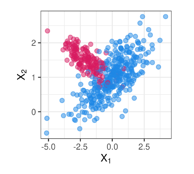
- LDA assumes linear boundaries, whereas QDA can capture quadratic curvature in the data.
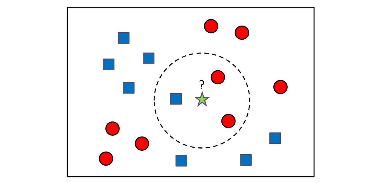
k-Nearest Neighbors (k-NN)
- \(k\)-NN is a non-parametric method that easily adapts to classification.
- Instead of assuming a parametric form for \(P(Y=c|\mathbf{x}=\dot{\mathbf{x}})\), it estimates this probability locally.
- The estimator of the posterior probability is the proportion of neighbors belonging to class \(c\): \[ \hat{P}(Y=c | \mathbf{x} = \dot{\mathbf{x}}_0) = \frac{1}{k} \sum_{i \in \mathcal{N}_{\dot{\mathbf{x}}_0}} I(y_i = c) \] where \(\mathcal{N}_{\dot{\mathbf{x}}_0}\) is the set of indices of the \(k\) training observations closest to the test point \(\dot{\mathbf{x}}_0\).
k-NN Classifier Details
- The plug-in classifier assigns \(\dot{\mathbf{x}}_0\) to the majority class among its neighbors: \[ \hat{f}(\dot{\mathbf{x}}_0) = \underset{c \in \mathcal{C}}{\text{arg max }} \hat{P}(Y=c | \mathbf{x} = \dot{\mathbf{x}}_0) \]
Thus, the predicted class of observation \(\dot{\mathbf{x}}_0\) is defined as:
\[ \hat{y}_0 = \underset{i \in \mathcal{N}_{\dot{\mathbf{x}}_0}}{\text{mode }} y_{i} \]
And how do we find the \(k\) nearest observations to \(\dot{\mathbf{x}}_0\)?
k-NN Distance Properties
- The \(k\)-NN Classifier selects the \(k\) nearest neighbors by calculating distances between training observations \(\dot{\mathbf{x}}_i\) and the test observation \(\dot{\mathbf{x}}_0\).
A distance function \(d(\dot{\mathbf{x}}_i, \dot{\mathbf{x}}_j)\) must satisfy the following properties:
\(d(\dot{\mathbf{x}}_i, \dot{\mathbf{x}}_j) \geq 0\) (Non-negativity);
\(d(\dot{\mathbf{x}}_i, \dot{\mathbf{x}}_j) = 0 \iff \dot{\mathbf{x}}_i = \dot{\mathbf{x}}_j\) (Identity of indiscernibles);
\(d(\dot{\mathbf{x}}_i, \dot{\mathbf{x}}_j) = d(\dot{\mathbf{x}}_j, \dot{\mathbf{x}}_i)\) (Symmetry);
\(d(\dot{\mathbf{x}}_i, \dot{\mathbf{x}}_j) \leq d(\dot{\mathbf{x}}_i, \dot{\mathbf{x}}_k) + d(\dot{\mathbf{x}}_k, \dot{\mathbf{x}}_j)\) (Triangle inequality).
k-NN Distance Metrics
The two most common distance metrics are the Euclidean distance and the Mahalanobis distance.
The Euclidean distance between two vectors \(\dot{\mathbf{x}}_i\) and \(\dot{\mathbf{x}}_j\) is given by:
\[d(\dot{\mathbf{x}}_i, \dot{\mathbf{x}}_j) = \sqrt{\sum_{l=1}^{p} (x_{il} - x_{jl})^2} = \sqrt{(\dot{\mathbf{x}}_i - \dot{\mathbf{x}}_j)^\top (\dot{\mathbf{x}}_i - \dot{\mathbf{x}}_j)}.\]
k-NN Distance Metrics
The Mahalanobis distance is given by:
\[d(\dot{\mathbf{x}}_i, \dot{\mathbf{x}}_j) = \sqrt{(\dot{\mathbf{x}}_i - \dot{\mathbf{x}}_j)^\top \hat{\boldsymbol{\Sigma}}^{-1} (\dot{\mathbf{x}}_i - \dot{\mathbf{x}}_j)},\] where \(\hat{\boldsymbol{\Sigma}}\) is the sample covariance matrix of the training data features.
k-NN: Key Practical Points
Important considerations:
- Scale Sensitivity: Euclidean distance is highly sensitive to the scale of variables. Features with large ranges will dominate the distance calculation. Thus, standardizing variables (to mean 0, variance 1) before running \(k\)-NN is crucial.
- Categorical Variables: Distances assume numeric features.
- Correlated Features: Mahalanobis distance is preferred when features are highly correlated, as it scales features according to their covariance structure.
k-NN Classifier Decision Boundaries
k-NN: Impact of \(k\)
Tree-Based Methods and Support Vector Machines
Classification Trees
- Classification Trees partition the feature space into a set of rectangular regions \(R_1, \dots, R_M\) and predict a constant class in each region. The predicted probability of class \(c\) in region \(R_m\) is the proportion of training instances in \(R_m\) that belong to class \(c\): \[ \hat{p}_{mc} = \frac{1}{|R_m|} \sum_{i \in R_m} I(y_i = c) \]
- To grow the tree, we recursively split regions. Splits are chosen to minimize impurity:
- Gini Impurity: \[ G = \sum_{c \in \mathcal{C}} \hat{p}_{mc} (1 - \hat{p}_{mc}) \]
- Entropy (Information Gain): \[ H = -\sum_{c \in \mathcal{C}} \hat{p}_{mc} \log \hat{p}_{mc} \]
Bagging and Random Forest
Tree models typically suffer from high variance. Ensemble methods mitigate this:
- Bagging (Bootstrap Aggregating):
- Generates \(B\) bootstrap samples from the training dataset. Fits an unpruned classification tree \(T_b(\dot{\mathbf{x}})\) on each sample.
- Combines predictions via majority vote: \[ \hat{f}_{\text{bag}}(\dot{\mathbf{x}}) = \underset{c \in \mathcal{C}}{\text{arg max }} \sum_{b=1}^B I(T_b(\dot{\mathbf{x}}) = c) \]
- Random Forest:
- Improves on Bagging by de-correlating the trees. At each node split, only a random subset of \(m \approx \sqrt{p}\) features is considered as candidates for the split.
- This prevents dominant features from making all bootstrap trees highly similar, further reducing ensemble variance.
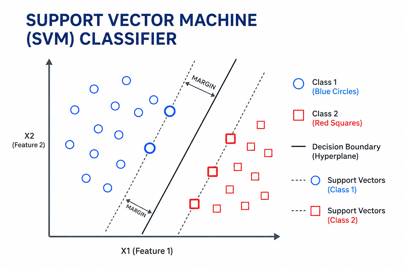
Support Vector Machines (SVM)
- Maximal Margin Classifier: If the classes are linearly separable, finds the separating hyperplane \(\boldsymbol{\beta}^\top \dot{\mathbf{x}} = 0\) that maximizes the margin (minimum distance from the hyperplane to any training point).
- Support Vector Classifier (Soft Margin): If classes are not perfectly separable, allows some points to violate the margin using slack variables \(\xi_i \ge 0\): \[ \max_{\boldsymbol{\beta}, \beta_0, \boldsymbol{\xi}} M \quad \text{subject to } y_i(\boldsymbol{\beta}^\top \dot{\mathbf{x}}_i) \ge M(1 - \xi_i), \quad \sum \xi_i \le C, \quad \xi_i \ge 0 \] where \(C\) is a budget for margin violations.
- Support Vector Machine: Extends the classifier to non-linear boundaries using the Kernel Trick. It projects features into a high-dimensional space where they become separable: \[ f(\dot{\mathbf{x}}) = \beta_0 + \sum_{i \in \mathcal{S}} \alpha_i y_i K(\dot{\mathbf{x}}_i, \dot{\mathbf{x}}) \] where \(\mathcal{S}\) is the set of support vectors and \(K(\cdot, \cdot)\) is a kernel (e.g., RBF kernel: \(\exp(-\gamma||\dot{\mathbf{x}}_i - \dot{\mathbf{x}}||^2)\)).
References
Basics
Aprendizado de Máquina: uma abordagem estatística, Izibicki, R. and Santos, T. M., 2020, link: https://rafaelizbicki.com/AME.pdf.
An Introduction to Statistical Learning: with Applications in R, James, G., Witten, D., Hastie, T. and Tibshirani, R., Springer, 2013, link: https://www.statlearning.com/.
Mathematics for Machine Learning, Deisenroth, M. P., Faisal. A. F., Ong, C. S., Cambridge University Press, 2020, link: https://mml-book.com.
References
Complementaries
An Introduction to Statistical Learning: with Applications in python, James, G., Witten, D., Hastie, T. and Tibshirani, R., Taylor, J., Springer, 2023, link: https://www.statlearning.com/.
Matrix Calculus (for Machine Learning and Beyond), Paige Bright, Alan Edelman, Steven G. Johnson, 2025, link: https://arxiv.org/abs/2501.14787.
Machine Learning Beyond Point Predictions: Uncertainty Quantification, Izibicki, R., 2025, link: https://rafaelizbicki.com/UQ4ML.pdf.
Mathematics of Machine Learning, Petersen, P. C., 2022, link: http://www.pc-petersen.eu/ML_Lecture.pdf.
Machine Learning - Prof. Jodavid Ferreira