Statistical Machine Learning
SVM
Maximal Margin Classifier
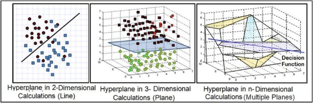
What Is a Hyperplane?
- In a \(p\)-dimensional space, a hyperplane is a flat affine subspace of dimension \(p-1\).
- In 2D: a line.
- In 3D: a plane.
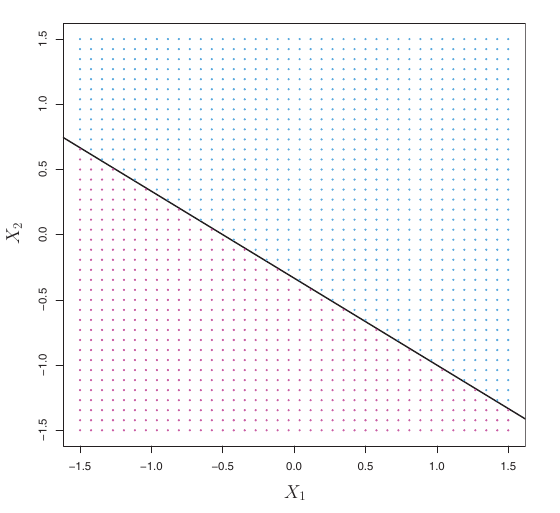
Hyperplanes for Classification
- If a point \(\mathbf{x}\) does not satisfy \(\beta_0 + \sum_{j=1}^p \beta_j X_j = 0\):
- If \(\beta_0 + \sum_{j=1}^p \beta_j X_j > 0\), \(X\) lies on one side of the hyperplane.
- If \(\beta_0 + \sum_{j=1}^p \beta_j X_j < 0\), \(X\) lies on the other side.
- A hyperplane divides \(p\)-dimensional space into two halves.
- We can determine which side a point lies on by the sign of \(f(\mathbf{x}) = \beta_0 + \sum_{j=1}^p \beta_j X_j\).
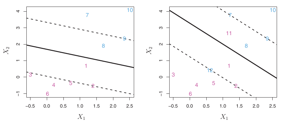
Infinite Separating Hyperplanes
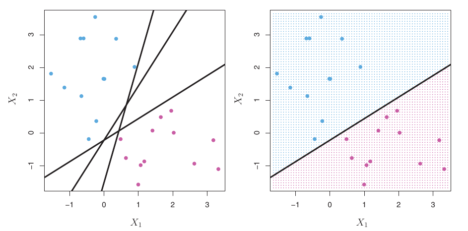
- If data is linearly separable, there are usually an infinite number of separating hyperplanes.
- A given separating hyperplane can often be shifted or rotated slightly without misclassifying any training points.
- Which one to choose? We need a systematic way to pick the “best” one.
The Maximal Margin Classifier (MMC)
The Non-Separable Case
- The MMC is great if a separating hyperplane exists.
- However, in many real-world datasets, classes are not perfectly linearly separable.
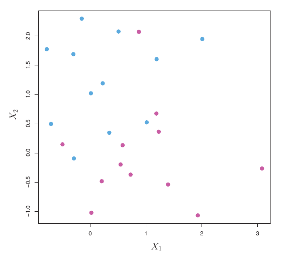
- In such cases, there is no solution to the MMC optimization problem with \(M > 0\).
- We need an extension that can handle overlapping classes. This leads to the Support Vector Classifier.
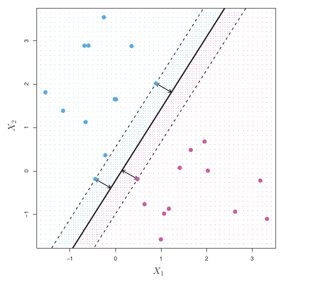
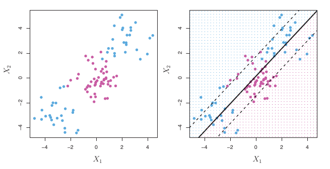
Support Vector Classifiers (SVC)

- Idea: Allow some observations to be on the wrong side of the margin, or even on the wrong side of the hyperplane (misclassified).
SVC: Allowing Violations
- The SVC aims for a hyperplane that separates most observations correctly, but tolerates some violations.
- This involves a trade-off:
- Wider margin (good for generalization).
- Fewer margin violations (good fit to training data).
- This is a bias-variance trade-off.
SVC: Role of \(C\)
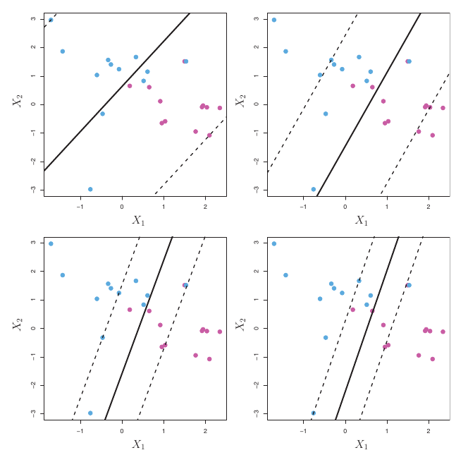
- Small C: Narrow margin, few violations allowed. Fits training data closely. Potentially high variance.
- Large C: Wider margin, more violations allowed. More robust to individual points. Potentially higher bias.
- This is a key way to control the bias-variance trade-off for SVC.
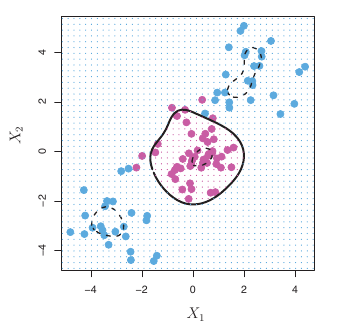
Support Vector Machines (SVM)
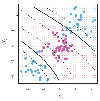
Classification with Non-linear Decision Boundaries
- SVCs produce linear decision boundaries.
- What if the true boundary is non-linear?
Common Kernels
Polynomial Kernel
- Polynomial Kernel of degree \(d\): \[ K(x_i, x_{i'}) = (1 + \sum_{j=1}^p x_{ij} x_{i'j})^d = (1 + \langle x_i, x_{i'} \rangle)^d \] where \(d\) is a positive integer (tuning parameter).
- Fits an SVM in a higher-dimensional space involving polynomials of degree \(d\).
- If \(d=1\), it’s similar to the linear kernel (though the \(1+\) term makes it slightly different).
- Can lead to much more flexible, non-linear decision boundaries.
Common Kernels:
Radial Basis Function (RBF) Kernel
- Radial Basis Function (RBF) Kernel (or Gaussian Kernel): \[ K(x_i, x_{i'}) = \exp \left( -\gamma \sum_{j=1}^p (x_{ij} - x_{i'j})^2 \right) = \exp(-\gamma \|x_i - x_{i'}\|^2_2) \] where \(\gamma > 0\) is a tuning parameter.
- Similarity \(K(x_i, x_{i'})\) is high if \(x_i\) and \(x_{i'}\) are close in Euclidean distance, and low if they are far.
- \(\gamma\) controls the “locality” or “reach” of the kernel.
- Small \(\gamma\): broader similarity, smoother boundary.
- Large \(\gamma\): more local similarity, potentially wigglier boundary.
- The feature space for RBF kernels is implicitly infinite-dimensional!