# Use ksmooth which implements Nadaraya-Watson
h_vals <- c(0.05, 0.2, 0.8) # Bandwidth h (span for ksmooth is different)
# ksmooth bandwidth 'h' corresponds to the full width 2h of the uniform kernel
# ksmooth 'bandwidth' argument seems different, maybe relates to h directly? Let's test.
x_grid <- seq(min(sim_data$x), max(sim_data$x), length.out = 100)
nw_preds_h <- list()

for (h_val in h_vals) {
  # Use kernel="box" for uniform
  fit <- ksmooth(x = sim_data$x, y = sim_data$y, kernel = "box", bandwidth = h_val, x.points = x_grid)
  nw_preds_h[[as.character(h_val)]] <- data.frame(x = fit$x, pred = fit$y, h = h_val)
}
nw_pred_h_df <- bind_rows(nw_preds_h)Statistical Machine Learning
Nonparametric Methods for Regression
Prof. Jodavid Ferreira
UFPE
Notation
- \(X\) or \(Y\)
- \(x\) or \(y\)
- \(\mathbf{x}\) or \(\mathbf{y}\)
- \(\dot{\mathbf{x}}\) or \(\dot{\mathbf{y}}\)
- \(\mathbf{X}\) or \(\mathbf{Y}\)
- \(\dot{\mathbf{X}}\) or \(\dot{\mathbf{Y}}\)
- \(p\)
- \(n\)
- \(i\)
- \(j\)
- \(k\)
represent random variables (r.v.);
represent realizations of random variables;
represent random vectors;
represent realizations of random vectors;
represent random matrices;
represent realizations of random matrices;
dimension of features, variables
sample size
\(i\)-th observation, instance (e.g., \(i=1, ..., n\))
\(j\)-th feature, variable, parameter (e.g., \(j=1, ..., p\))
number of neighbors (KNN) or folds (CV)
k-Nearest Neighbors (KNN) Regression
k-Nearest Neighbors (KNN)
Regression
Core Idea:
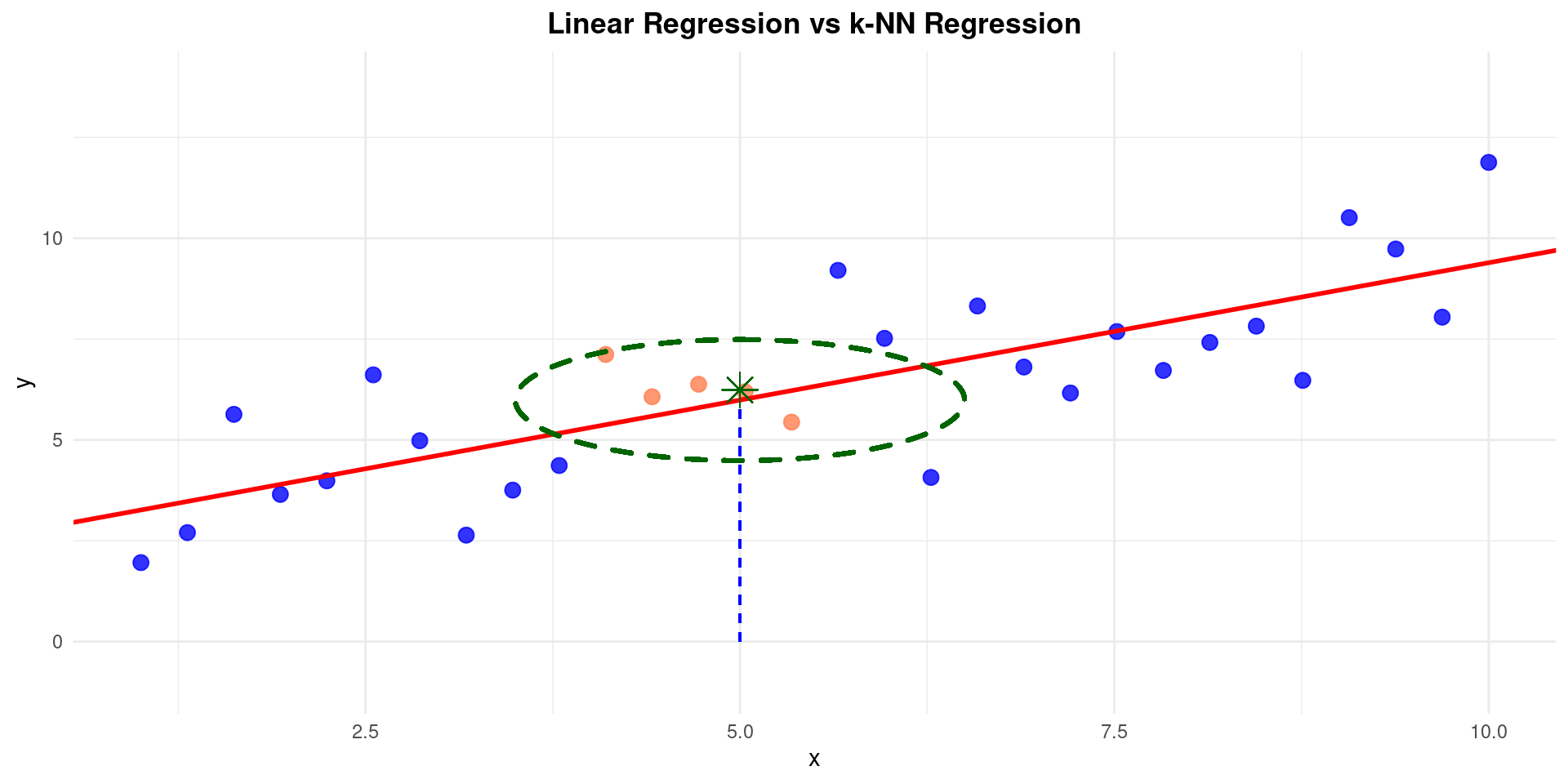
- To predict the response at a point \(\dot{\mathbf{x}}\), find the \(k\) training observations \((\dot{\mathbf{x}}_i, y_i)\) whose features \(\dot{\mathbf{x}}_i\) are closest to \(\mathbf{x}\). Average their responses \(y_i\).
One of the simplest nonparametric methods.
Given:
- A target point \(\mathbf{x}\) (where we want to predict \(f(\mathbf{x})\)).
- A distance metric \(d(\dot{\mathbf{x}}_i, \dot{\mathbf{x}}_j)\) (e.g., Euclidean distance).
- The training data \(\{ (\dot{\mathbf{x}}_i, y_i) \}_{i=1}^n\).
- The number of neighbors \(k\).
k-Nearest Neighbors (KNN)
Regression
Find the set \(\mathcal{N}_{\mathbf{x}}\) containing the indices of the \(k\) points \(\dot{\mathbf{x}}_i\) in the training set that are closest to \(\mathbf{x}\) according to the distance metric. \[ \mathcal{N}_{\mathbf{x}} = \{ i \in \{1, \ldots, n\} \mid \dot{\mathbf{x}}_i \text{ is one of the } k \text{ closest points to } \mathbf{x} \} \]
(Let \(d_{(k)}(\mathbf{x})\) be the distance to the k-th nearest neighbor of \(\mathbf{x}\). Then \(\mathcal{N}_{\mathbf{x}} = \{i \mid d(\dot{\mathbf{x}}_i, \mathbf{x}) \le d_{(k)}(\mathbf{x}) \}\), handling ties appropriately).*
- The KNN regression estimate is the average of the responses for these neighbors: \[ \hat{f}_k(\mathbf{x}) = \frac{1}{k} \sum_{i \in \mathcal{N}_{\mathbf{x}}} y_i \]
k-Nearest Neighbors (KNN)
Regression
Assumes that points close together in the predictor space \(\mathcal{X}\) likely have similar response values \(Y\).
Forms a local neighborhood and calculates a simple local average.
The “model” is just the training data itself. Prediction requires searching through the data.

k-Nearest Neighbors (KNN)
Regression
k-Nearest Neighbors (KNN)
Tuning Parameter \(k\)
The \(k\) value is the number of neighbors, is the main tuning parameter.
- Bias-Variance Trade-off for \(k\):
Small \(k\) (e.g., \(k=1\)):
Low bias (uses only the very closest points).
High variance (prediction is sensitive to noise in the single nearest neighbor).
Large \(k\) (e.g., \(k=n\)):
- High bias (averages over many potentially dissimilar points; tends towards the global mean of \(Y\)).
- Low variance (average of many points is stable). Very smooth fit (constant if \(k=n\)).
- \(k\) is typically chosen using cross-validation.
k-Nearest Neighbors (KNN)
(Influence of \(k\))
Let’s revisit the 1D simulated data.
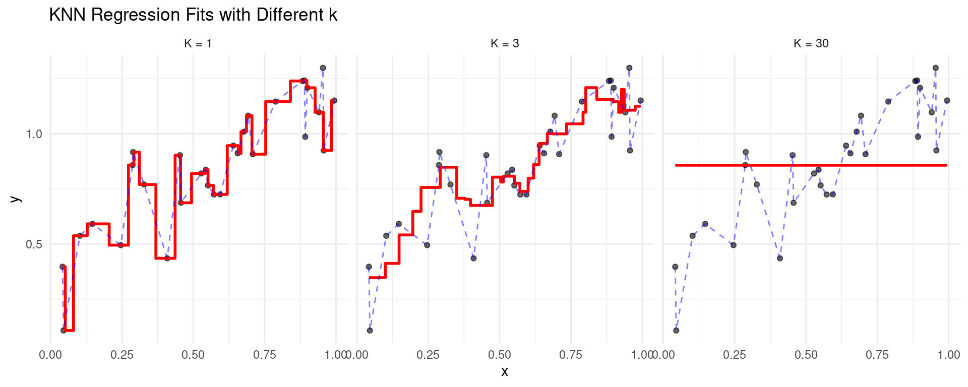
Note the characteristic “step function” appearance of KNN regression.
k-Nearest Neighbors (KNN)
(Curse of Dimensionality)
- KNN works reasonably well in low dimensions (\(p\) small).
- In high dimensions (\(p\) large), the concept of “nearest neighbors” becomes less meaningful.
- All points tend to be far away from each other.
- The volume of the neighborhood needed to capture \(k\) points grows rapidly.
- Points within the neighborhood may not be truly “local” in all dimensions.
- Requires exponentially more data to maintain the density of points as \(p\) increases.
- This is a major limitation of KNN in high-dimensional settings. Predictor scaling becomes very important.
Nadaraya-Watson Kernel Regression
Nadaraya-Watson Kernel Regression
- A variation/improvement on KNN. Also based on local averaging, but uses a smooth weighting scheme instead of a hard cutoff.
- Proposed independently by Nadaraya (1964) and Watson (1964).
Core Idea:
- Assign weights \(w_i(\mathbf{x})\) to each training point \((\dot{\mathbf{x}}_i, y_i)\) based on how close \(\dot{\mathbf{x}}_i\) is to the target point \(\mathbf{x}\). Points closer to \(\mathbf{x}\) get higher weights. \[ \hat{f}(\mathbf{x}) = \sum_{i=1}^n w_i(\mathbf{x}) y_i \]
Nadaraya-Watson Kernel Regression
Weights
The weights are defined using a kernel function \(K\) and a bandwidth \(h\):
\[ w_i(\mathbf{x}) = \frac{K_h(d(\mathbf{x}, \dot{\mathbf{x}}_i))}{\sum_{j=1}^n K_h(d(\mathbf{x}, \dot{\mathbf{x}}_j))} \]
where \(K_h(u) = K(u/h)\) is the scaled kernel function, \(K\) is the kernel profile (a non-negative function, usually symmetric around 0, integrating to 1), and \(d(\mathbf{x}, \dot{\mathbf{x}}_i)\) is the distance.
- The weights sum to 1: \(\sum_{i=1}^n w_i(\mathbf{x}) = 1\).
- The estimator is a weighted average of the responses \(y_i\).
Kernel Functions \(K(u)\)
The kernel function \(K(u)\) determines the shape of the weights. Common choices (for \(u \ge 0\), assuming distance \(d \ge 0\); often defined for \(u=d/h\)):
- Uniform (Boxcar): \(K(u) = \frac{1}{2} \mathbb{I}(|u| \le 1)\)
- Equivalent to KNN within distance \(h\). Assigns equal weight to neighbors within distance \(h\), zero weight outside. \[ K_h(d(\mathbf{x}, \dot{\mathbf{x}}_i)) \propto \mathbb{I}(d(\mathbf{x}, \dot{\mathbf{x}}_i) \le h) \]
- Triangular: \(K(u) = (1 - |u|) \mathbb{I}(|u| \le 1)\)
- Linearly decreasing weights. \[ K_h(d(\mathbf{x}, \dot{\mathbf{x}}_i)) \propto (1 - d(\mathbf{x}, \dot{\mathbf{x}}_i)/h) \mathbb{I}(d(\mathbf{x}, \dot{\mathbf{x}}_i) \le h) \]
Kernel Functions \(K(u)\)
- Epanechnikov: \(K(u) = \frac{3}{4} (1 - u^2) \mathbb{I}(|u| \le 1)\)
- Parabolic weights. Optimal in terms of minimizing asymptotic MSE. \[ K_h(d(\mathbf{x}, \dot{\mathbf{x}}_i)) \propto (1 - (d(\mathbf{x}, \dot{\mathbf{x}}_i)/h)^2) \mathbb{I}(d(\mathbf{x}, \dot{\mathbf{x}}_i) \le h) \]
- Gaussian: \(K(u) = \frac{1}{\sqrt{2\pi}} e^{-u^2/2}\)
- Smoothly decreasing weights, assigns non-zero (but potentially tiny) weight to all points. \[ K_h(d(\mathbf{x}, \dot{\mathbf{x}}_i)) \propto \exp\left(-\frac{d(\mathbf{x}, \dot{\mathbf{x}}_i)^2}{2h^2}\right) \]
Bandwidth \(h\): The Tuning Parameter
The bandwidth \(h > 0\) controls the width of the kernel, determining the size of the local neighborhood being averaged over.
- Bias-Variance Trade-off for \(h\):
- Small \(h\): Narrow kernel, uses only very close points.
- Low bias.
- High variance (wiggly fit).
- Large \(h\): Wide kernel, averages over a large region.
- High bias (oversmoothed fit).
- Low variance.
- Small \(h\): Narrow kernel, uses only very close points.
- \(h\) is the crucial tuning parameter, typically chosen via cross-validation.
- The choice of kernel shape (\(K\)) usually has a smaller impact on performance than the choice of bandwidth \(h\).
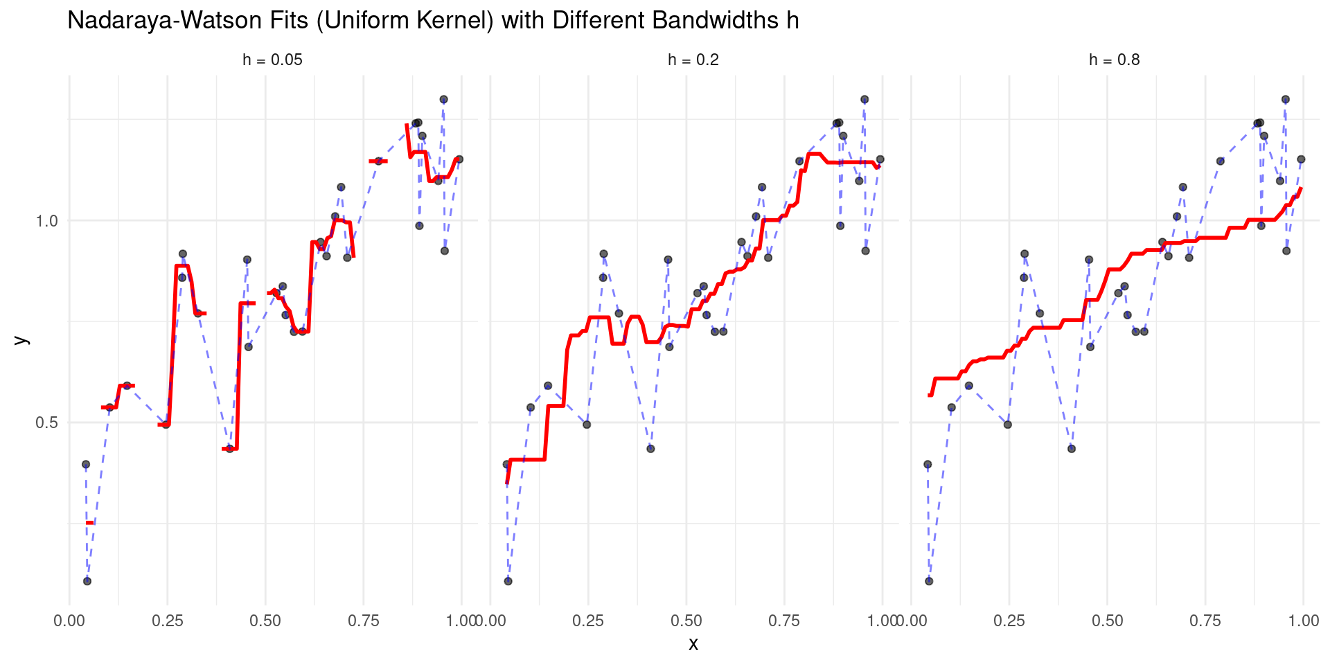
Nadaraya-Watson Visualization
Influence of \(h\)
Using the Uniform kernel.
Nadaraya-Watson Visualization
Influence of \(h\)
Using the Uniform kernel.
Nadaraya-Watson Visualization
Influence of Kernel
Comparing Uniform (“box”) and Gaussian (“normal”) kernels with the same bandwidth \(h=0.1\).
h_fixed <- 0.1
kernels <- c("box", "normal")
nw_preds_k <- list()

for (k_name in kernels) {
  fit <- ksmooth(x = sim_data$x, y = sim_data$y, kernel = k_name, bandwidth = h_fixed, x.points = x_grid)
  nw_preds_k[[k_name]] <- data.frame(x = fit$x, pred = fit$y, kernel = k_name)
}
nw_pred_k_df <- bind_rows(nw_preds_k)- Gaussian kernel gives a smoother result than the uniform kernel.
Nadaraya-Watson Visualization
Influence of Kernel
Comparing Uniform (“box”) and Gaussian (“normal”) kernels with the same bandwidth \(h=0.1\).
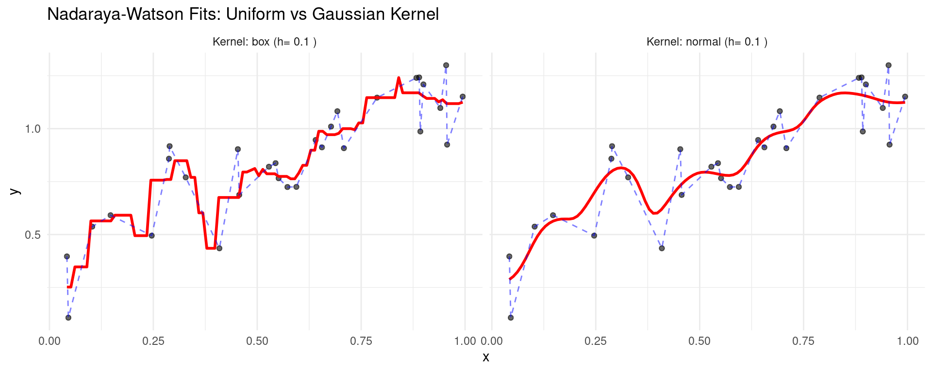
- Gaussian kernel gives a smoother result than the uniform kernel.
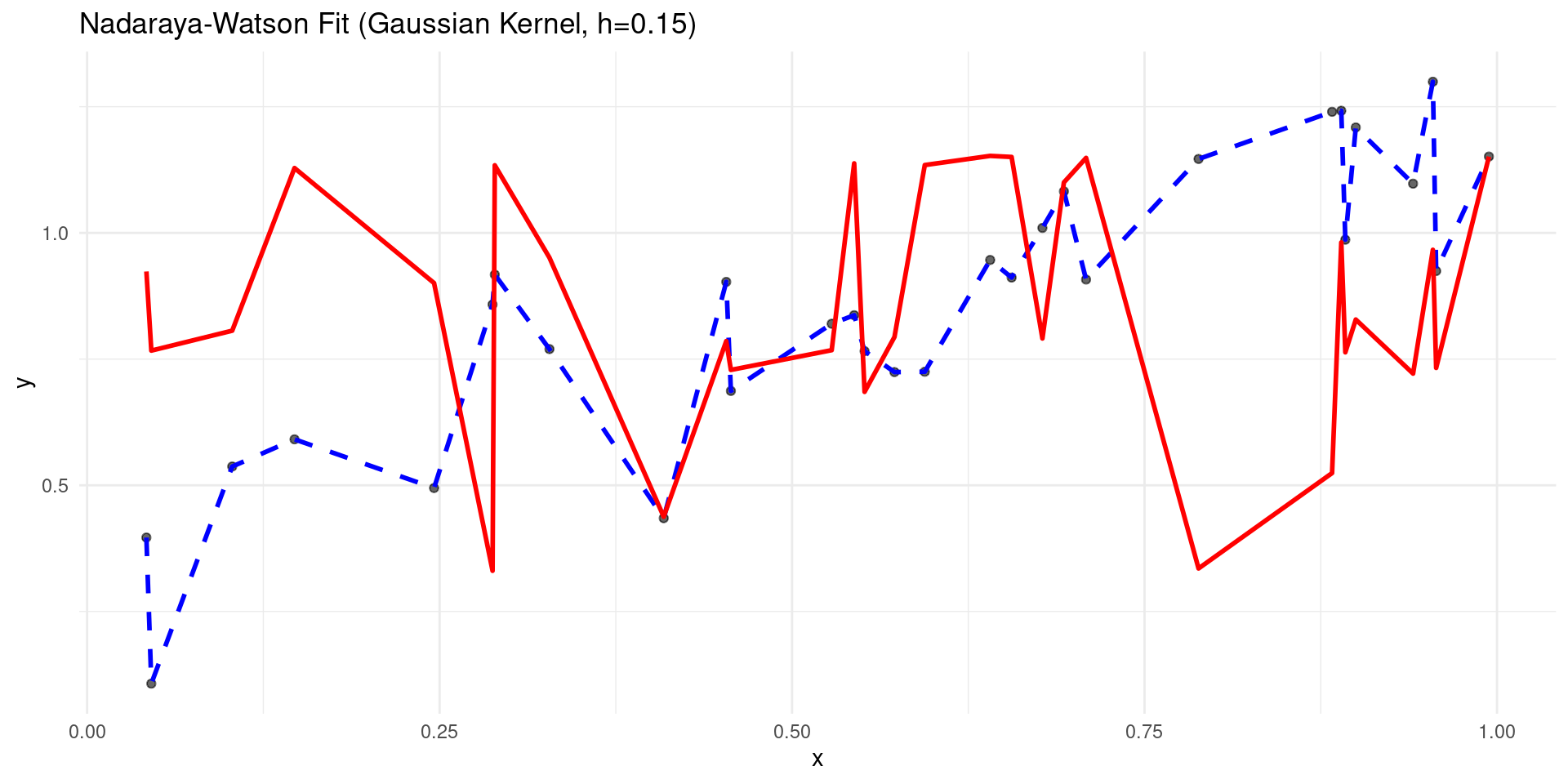
R Example: Nadaraya-Watson
ksmooth
R’s stats::ksmooth function performs Nadaraya-Watson regression.
# Using ksmooth
h_choice <- 0.15 # Chosen via CV, perhaps
fit_ks <- ksmooth(x = sim_data$x, y = sim_data$y,
                  kernel = "normal", # Gaussian kernel
                  bandwidth = h_choice,
                  x.points = sim_data$x) # Predict at original points

sim_data$pred_ksmooth <- fit_ks$y

p <- ggplot(sim_data, aes(x = x)) +
  geom_point(aes(y = y), alpha = 0.6) +
  geom_line(aes(y = y_true), color = "blue", linewidth = 1, linetype = "dashed") +
  geom_line(aes(y = pred_ksmooth), color = "red", linewidth = 1) +
  labs(title = paste("Nadaraya-Watson Fit (Gaussian Kernel, h=", h_choice, ")", sep="")) +
  theme_minimal()
R Example: Nadaraya-Watson
ksmooth
R’s stats::ksmooth function performs Nadaraya-Watson regression.
Summary: Methods Covered
k-Nearest Neighbors (KNN): Predict using the average response of the \(k\) closest training points. Simple, intuitive, but can be slow and sensitive to \(p\).
Nadaraya-Watson: Predict using a weighted average, with weights determined by a kernel function \(K\) and bandwidth \(h\).
All these methods involve tuning parameters (\(k\) or \(h\)) that control the bias-variance trade-off.
Cross-validation is essential for choosing these parameters.
Understanding the underlying assumptions and trade-offs is key to applying these methods effectively.
References
Basics
Aprendizado de Máquina: uma abordagem estatística, Izibicki, R. and Santos, T. M., 2020, link: https://rafaelizbicki.com/AME.pdf.
An Introduction to Statistical Learning: with Applications in R, James, G., Witten, D., Hastie, T. and Tibshirani, R., Springer, 2013, link: https://www.statlearning.com/.
Mathematics for Machine Learning, Deisenroth, M. P., Faisal. A. F., Ong, C. S., Cambridge University Press, 2020, link: https://mml-book.com.
References
Complementaries
An Introduction to Statistical Learning: with Applications in python, James, G., Witten, D., Hastie, T. and Tibshirani, R., Taylor, J., Springer, 2023, link: https://www.statlearning.com/.
Matrix Calculus (for Machine Learning and Beyond), Paige Bright, Alan Edelman, Steven G. Johnson, 2025, link: https://arxiv.org/abs/2501.14787.
Machine Learning Beyond Point Predictions: Uncertainty Quantification, Izibicki, R., 2025, link: https://rafaelizbicki.com/UQ4ML.pdf.
Mathematics of Machine Learning, Petersen, P. C., 2022, link: http://www.pc-petersen.eu/ML_Lecture.pdf.
Machine Learning - Prof. Jodavid Ferreira